Dimensionality Reduction: Motivation and Problem Setup

David I. Inouye

Dimensionality Reduction: Motivation and Problem Setup

A table can be computable while remaining impossible to inspect

Suppose we measure 20,000 gene-expression values for each of 500 cells.

\(500\) cells \(\times\) \(20{,}000\) measurements per cell

  • A computer can store and manipulate the table.
  • A person cannot directly see its geometry in 20,000 dimensions.
  • We still want to find groups of similar cells, flag unusual cells, reveal related or connected structures, and remove statistical noise.

Dimensionality reduction serves two practical goals

1. Visualize hidden structure

Create a 2D view where we can look for:

  • clusters of similar cells;
  • unusual cells or outliers; and
  • connected, branching, or other structures.

2. Improve further analysis

Create a lower-dimensional representation that:

  • requires less computation; and
  • can yield more reliable statistical estimates by ignoring spurious variation caused by finite samples or measurement noise.

Both goals replace many measured features with fewer useful features.

Goal 1: visualize hidden structure

Original observations

  • One point per cell
  • Thousands of measured features
  • Structure exists beyond direct human vision

Illustrative two-dimensional scatter plot with several groups of nearby points

This is a representation of handwritten digits—not cells—but it illustrates the kinds of clusters and other structure we might seek in cellular data.

Goal 2: improve further analysis

A lower-dimensional representation can provide:

  • computational efficiency: fewer features to store and process;
  • statistical efficiency: fewer irrelevant directions to estimate from limited data; and
  • denoising: less sensitivity to measurement noise or spurious sample variation.

These benefits require the discarded variation to be less useful than the structure retained. Reduction is not automatically an improvement.

Both goals lead to the problem of dimensionality reduction

We seek a new representation with far fewer features:

high-dimensional observations \(\longrightarrow\) low-dimensional representation

But “make it simpler” does not say what a faithful simplification should retain.

  • Which points should remain near one another?
  • Which directions of spread should remain large?
  • Which distinctions may be treated as noise?
  • Should the original measurements be approximately recoverable?

What kind of structure do we want to maintain?

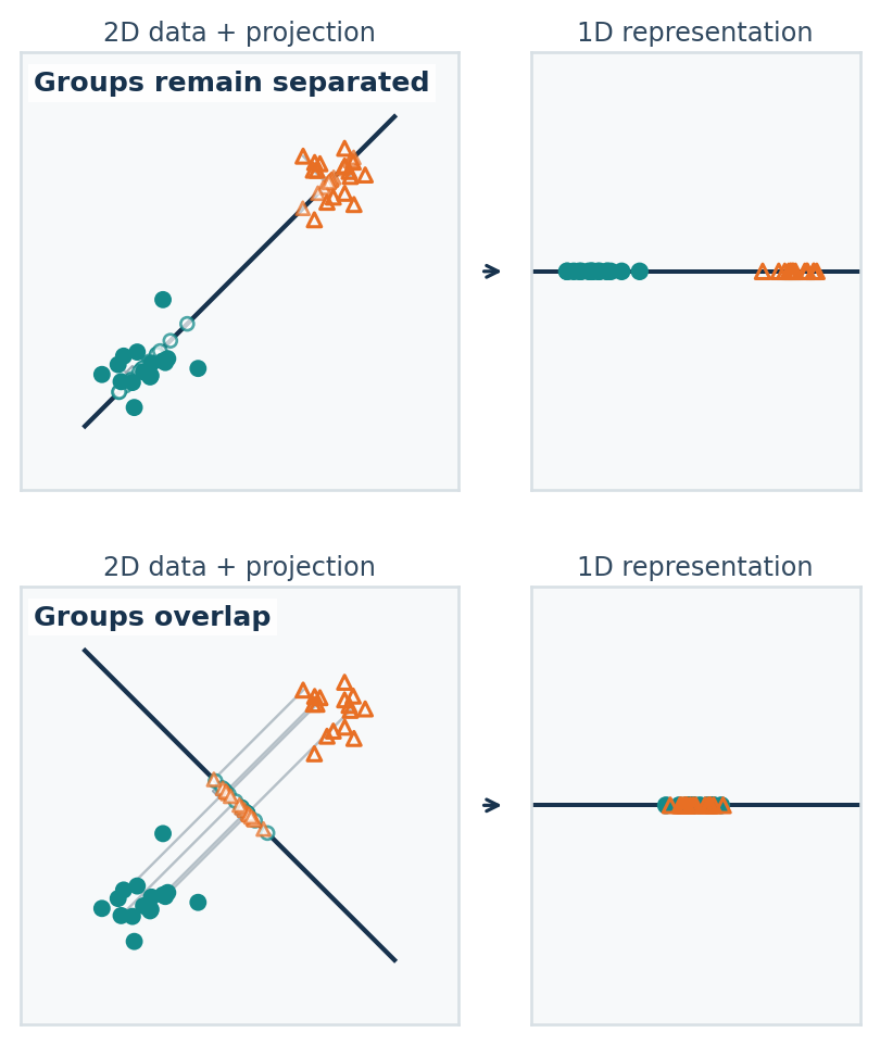
The same two groups of two-dimensional points projected onto two different lines. One one-dimensional representation keeps the groups apart; the other makes them overlap. Light perpendicular paths show selected points projected onto each line.

Groups and neighborhoods. Keep nearby points close and distinct groups separate when those relationships matter.

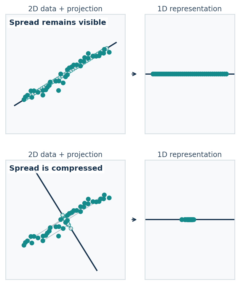
The same elongated cloud of two-dimensional points projected along and across its main direction. One one-dimensional representation retains substantial spread; the other compresses the points together. Light perpendicular paths show selected projections.

Spread. Retain directions in which the observations vary rather than compressing meaningful variation.

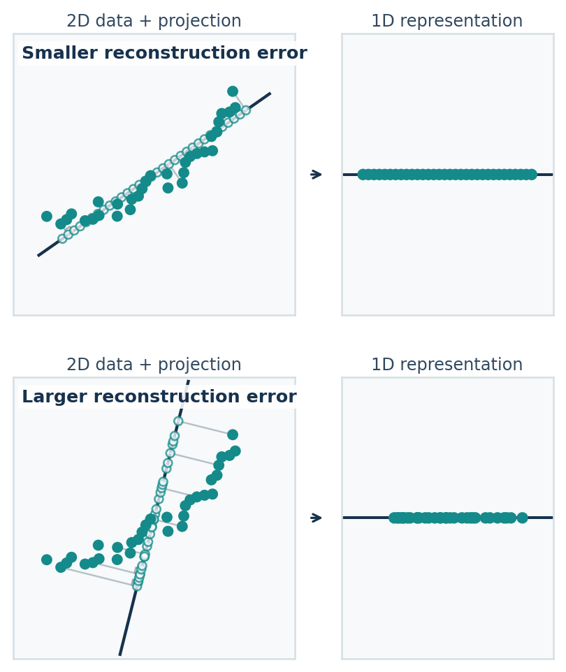
The same slightly curved noisy two-dimensional data projected onto two different lines. A well-aligned line leaves short perpendicular reconstruction errors; a poorly aligned line leaves longer errors. Each projection also produces a one-dimensional representation.

Reconstruction. Prefer features that can recover points close to their original 2D locations when reconstruction matters.

How do we formalize these criteria?

We need the language of vectors, geometry, and linear transformations.

Formalization starts by naming one observation

For cell \(i\), collect its \(d\) measured features into a vector:

\[ \boldsymbol{x}_i = \begin{bmatrix} x_{i1} & x_{i2} & \cdots & x_{id} \end{bmatrix}^{T} \in \mathbb{R}^{d} \]

  • \(i\) identifies the cell.
  • \(j\) identifies a measured feature such as one gene.
  • \(d\) is the number of observed features—not automatically the number of meaningful directions in the data.

A data matrix records features—not intrinsic dimension

Stack \(n\) observations as rows:

\[ X = \begin{bmatrix} ---\boldsymbol{x}_1^T---\\ ---\boldsymbol{x}_2^T---\\ \vdots\\ ---\boldsymbol{x}_n^T--- \end{bmatrix} \in \mathbb{R}^{n\times d} \]

rows \(=\) observations
columns \(=\) measured features

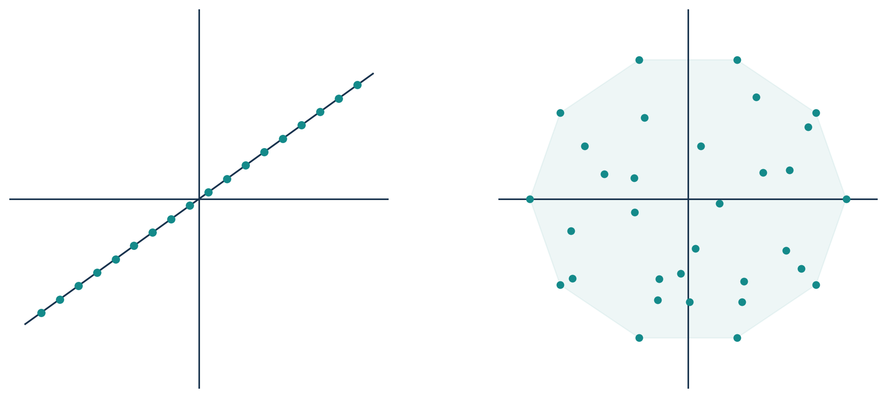
1D structure in 2D

2D structure in 2D

Two coordinate planes: points on the left lie on one diagonal line while points on the right spread across a two-dimensional region

Both datasets have two measured features; only one needs two independent directions to describe its variation.

We seek a function from observed to reduced features

For each observation, seek

\[ f:\mathbb{R}^{d}\rightarrow\mathbb{R}^{k}, \qquad \boldsymbol{z}_i=f(\boldsymbol{x}_i), \qquad k\ll d, \]

where \(\boldsymbol{x}_i\in\mathcal{X}\subseteq\mathbb{R}^{d}\) contains the observed features and \(\boldsymbol{z}_i\in\mathcal{Z}\subseteq\mathbb{R}^{k}\) contains the reduced features.

For now, assume \(f\) is linear. Later, we will learn nonlinear representation functions—but linear transformations are the foundation for analyzing both.

To define, analyze, and choose this \(f\), we need linear algebra for geometry, transformations, and lower-dimensional structure.

The problem organizes what comes next

We began with a need: make high-dimensional relationships inspectable without pretending every relationship survives.

We now have:

  1. an explicit purpose and candidate preservation criteria;
  2. observations \(\boldsymbol{x}_i\), a data matrix \(X\), and desired reduced features \(Z\);
  3. a visual distinction among neighborhoods, spread, and reconstruction; and
  4. a concrete reason to develop the linear algebra needed to finish the model.