Linear Transformations: What Do They Do?

David I. Inouye

Dynamic Content · Last Updated: September 11, 2026

This topic treats a matrix as a transformation between feature spaces. Keep the 1D scalar analogy visible throughout. SVD explains directional scaling, rank, null space, and recovery within this topic. Reconstruction and PCA form the next topic.

A linear representation turns the problem into a matrix question

We began with a representation function:

\[ f:\mathbb{R}^{d}\rightarrow\mathbb{R}^{m}, \qquad \boldsymbol{y}=f(\boldsymbol{x}). \]

For this first representation model, assume \(f\) is linear:

\[ \boldsymbol{y}=A\boldsymbol{x}, \qquad A\in\mathbb{R}^{m\times d}. \]

What can this transformation do to a high-dimensional feature space?

Reconnect to the previous topic without repeating its full setup. The symbols change from reduced features z to generic output features y because this topic studies any linear transformation, including ones that increase dimension.

Matrix multiplication generalizes scalar multiplication

One dimension

\[ y=ax \]

• \(x,y,a\) are scalars.
• \(a\) scales one number line.
• The sign can reverse direction.

Higher dimensions

\[ \boldsymbol{y}=A\boldsymbol{x} \]

• \(\boldsymbol{x}\) and \(\boldsymbol{y}\) are vectors.
• \(A\) can scale different directions differently.
• Input and output can have different dimensions.

\(a\) becomes \(A\): one scalar action becomes a transformation of a feature space.

Use this correspondence repeatedly. Do not imply that A merely scales the coordinate axes as written; the later SVD shows the directions in which the independent scalar actions occur.

Each output feature receives a weighted connection from every input

\[ A= \begin{bmatrix} 2 & -1 & 0.5\\ 1 & 0 & -2 \end{bmatrix} \]

• A teal edge contributes to \(y_1\).
• An orange edge contributes to \(y_2\).
• Every edge weight is one entry \(a_{ji}\).

Trace one input value along both outgoing edges. The diagram resembles a neural network, but do not introduce that term yet. Its purpose is to make an ordinary matrix multiplication visible as weighted connections.

Every output is a different linear combination of the inputs

\[ \begin{aligned} y_1 &=2x_1-x_2+0.5x_3\\ &=2(1)-2+0.5(-1)\\ &=-0.5 \end{aligned} \]

\[ \begin{aligned} y_2 &=x_1+0x_2-2x_3\\ &=1+0-2(-1)\\ &=3 \end{aligned} \]

\[ \underbrace{ \begin{bmatrix}-0.5\\3\end{bmatrix} }_{\boldsymbol{y}} = \underbrace{ \begin{bmatrix}2&-1&0.5\\1&0&-2\end{bmatrix} }_{A} \underbrace{ \begin{bmatrix}1\\2\\-1\end{bmatrix} }_{\boldsymbol{x}} \]

First read each scalar equation. On reveal, align each equation with one row of A. Row-by-column multiplication is the mechanism; the weighted combination is its meaning.

One matrix applies the same transformation to every observation

For observation \(i\):

\[ \boldsymbol{y}_i=A\boldsymbol{x}_i, \qquad \boldsymbol{x}_i\in\mathbb{R}^{d}, \quad \boldsymbol{y}_i\in\mathbb{R}^{m}. \]

The same entries of \(A\) define every output feature for every observation.

• Convention: Vectors such as \(\boldsymbol{x}_i\) are usually written as columns.
• Transpose: \(A^T\) swaps rows and columns: \(A\in\mathbb{R}^{m\times d}\Rightarrow A^T\in\mathbb{R}^{d\times m}\).

One linear operator gives a consistent representation rule for the entire dataset.

Prepare the batch activity without yet displaying its answer. Emphasize that A contains parameters of the representation, while each observation supplies new input values.

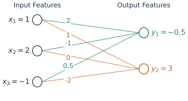
Which batch equation has the right shape?

Observations are rows:

\[ X=\begin{bmatrix} 1&2&-1\\ 0&1&2\\ 2&-1&1 \end{bmatrix} \]

Use the same transformation:

\[ A=\begin{bmatrix} 2&-1&0.5\\ 1&0&-2 \end{bmatrix} \]

Compute \(Y\) with one matrix multiplication

\[Y=\text{???}\]

\[ \underbrace{Y}_{3\times2} =\underbrace{X}_{3\times3}\underbrace{A^T}_{3\times2} =\begin{bmatrix} -0.5&3\\ 0&-4\\ 5.5&0 \end{bmatrix} \]

Each row of \(Y\) is \((A\boldsymbol{x}_i)^T\).

Activity, about 2 minutes. Ask students to construct the batch equation and predict its shape before revealing the answer. A strong response checks the inner dimensions and reconciles column-vector mathematics with row-stacked data.

Matrix algebra preserves some scalar rules and rejects others

Valid for scalars and matrices

\[ A(B\boldsymbol{x})=(AB)\boldsymbol{x} \]

\[ A(\boldsymbol{x}+\boldsymbol{z}) =A\boldsymbol{x}+A\boldsymbol{z} \]

\[ AI=A \]

Order matters for matrices

\[ AB\ne BA \quad \text{in general} \]

\[ (AB)^T=B^TA^T \]

Changing the order can change the value or make the product undefined.

Students do not need the property names as vocabulary targets. They do need to know which rearrangements preserve an equation. Contrast scalar commutativity with matrix order and point out that dimensions often expose an invalid move.

Dimensions expose many invalid manipulations

Let \(A\in\mathbb{R}^{m\times d}\) and \(B\in\mathbb{R}^{d\times p}\).

Valid

\[ AB\in\mathbb{R}^{m\times p} \]

\[ (AB)^T=B^TA^T \]

Not guaranteed to exist

\[ BA \]

The inner dimensions would require \(p=m\).

Shape is part of the mathematical claim, not an implementation detail.

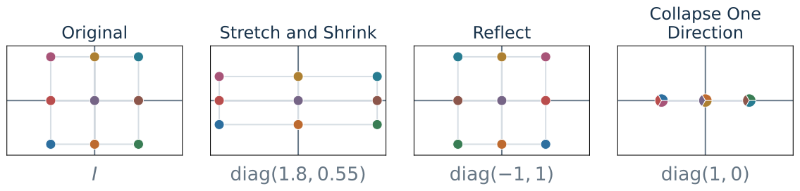
A diagonal matrix applies a separate 1D scaling to each feature

Colors track the same inputs. Three colored sectors at one output location show that three inputs have collapsed together.

Connect each diagonal entry to an independent scalar multiplier. The final panel previews singularity without generalizing it yet: after SVD, any matrix with a zero singular value will contain this same irreversible action in some direction.

The Euclidean norm measures size and distance

For \(\boldsymbol{x}\in\mathbb{R}^{d}\):

\[ \lVert\boldsymbol{x}\rVert_2 =\sqrt{x_1^2+x_2^2+\cdots+x_d^2} \]

For two points \(\boldsymbol{x}_i\) and \(\boldsymbol{x}_j\):

\[ \operatorname{dist}(\boldsymbol{x}_i,\boldsymbol{x}_j) =\lVert\boldsymbol{x}_i-\boldsymbol{x}_j\rVert_2 \]

The subscript \(2\) identifies the Euclidean norm. Other norms measure size differently.

This is the only norm needed now. Keep L1 and infinity norms for later problems where their different geometry or robustness matters.

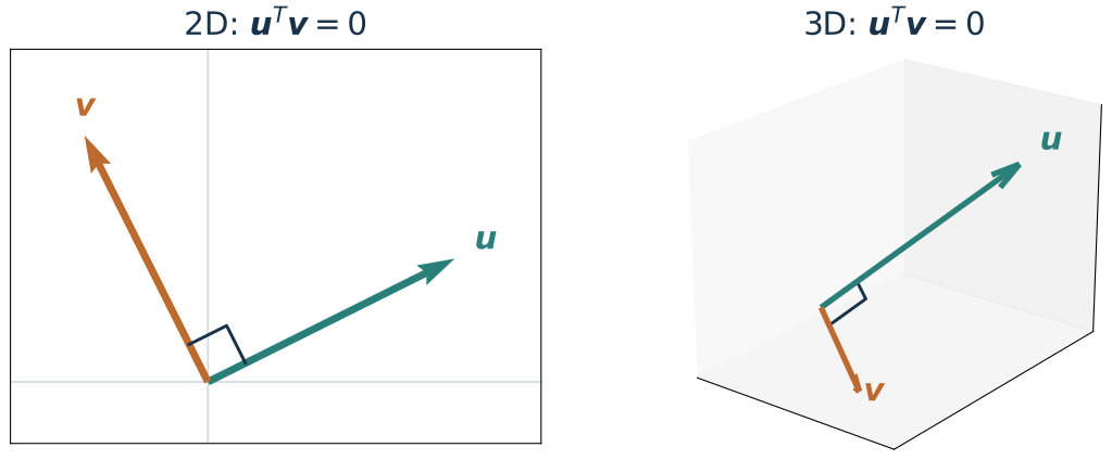
Orthogonal vectors meet at a right angle

\[ \boldsymbol{u}\perp\boldsymbol{v} \quad\Longleftrightarrow\quad \boldsymbol{u}^{T}\boldsymbol{v}=0 \]

Define the perpendicular symbol before using it. In two and three dimensions, students can see a right angle. The zero inner product is the definition that continues to work when a picture is impossible.

In higher dimensions, we compute orthogonality

Are these dense five-dimensional vectors orthogonal?

\[ \boldsymbol{u}=\begin{bmatrix}1\\2\\-1\\3\\4\end{bmatrix}, \qquad \boldsymbol{v}=\begin{bmatrix}2\\-1\\3\\2\\-\tfrac34\end{bmatrix} \]

\[ \boldsymbol{u}^{T}\boldsymbol{v} =2-2-3+6-3 =0 \qquad\Longrightarrow\qquad \boldsymbol{u}\perp\boldsymbol{v} \]

Orthogonality is defined in any dimension, even when geometry cannot be visualized.

Pause before revealing the dot product. Every coordinate is nonzero, and no visual inspection makes the relationship obvious. This is why the algebraic definition matters in high-dimensional spaces.

An orthogonal matrix has orthonormal columns

For a square matrix \(Q=[\boldsymbol{q}_1\;\cdots\;\boldsymbol{q}_d]\in\mathbb{R}^{d\times d}\), orthonormal means mutually orthogonal columns, each of unit length.

Higher dimensions	Interpretation	1D special case	Interpretation
\(I\boldsymbol{x}=\boldsymbol{x}\)	The identity matrix leaves a vector unchanged.	\(1x=x\)	The scalar \(1\) leaves a number unchanged.
\((Q^TQ)_{ij}=\boldsymbol{q}_i^T\boldsymbol{q}_j\)	Multiplication collects all column inner products.	\(q\,q=q^2\)	There is only one entry to multiply by itself.
\(Q^TQ=I\)	Inner products are \(1\) for the same column, \(0\) for distinct columns.	\(q^2=1\)	Hence \(q\in\{-1,1\}\).
\(\boldsymbol{y}=Q\boldsymbol{x}\)	Rotates or reflects about the origin, preserving length.	\(y=qx\)	Keeps or reverses direction while preserving length.

Introduce the higher-dimensional definition first, then read each row from left to right to connect it to the 1D special case Q = [q]. The identity matrix plays exactly the role of 1. Q transpose Q is the table of column inner products: the diagonal entries are squared column lengths, and off-diagonal entries test orthogonality. In 1D, transpose changes nothing and the condition reduces to q squared equals one. The final row previews the geometric interpretation; the next two slides ask students to predict distance preservation and prove it.

Do orthogonal transformations preserve every pairwise distance?

Is \(\lVert Q\boldsymbol{x}_i-Q\boldsymbol{x}_j\rVert_2\) equal to \(\lVert\boldsymbol{x}_i-\boldsymbol{x}_j\rVert_2\) for every pair?

Pause for a prediction. The entire configuration appears rotated and reflected; the highlighted segments make several pairwise comparisons visible without claiming that only those pairs are preserved.

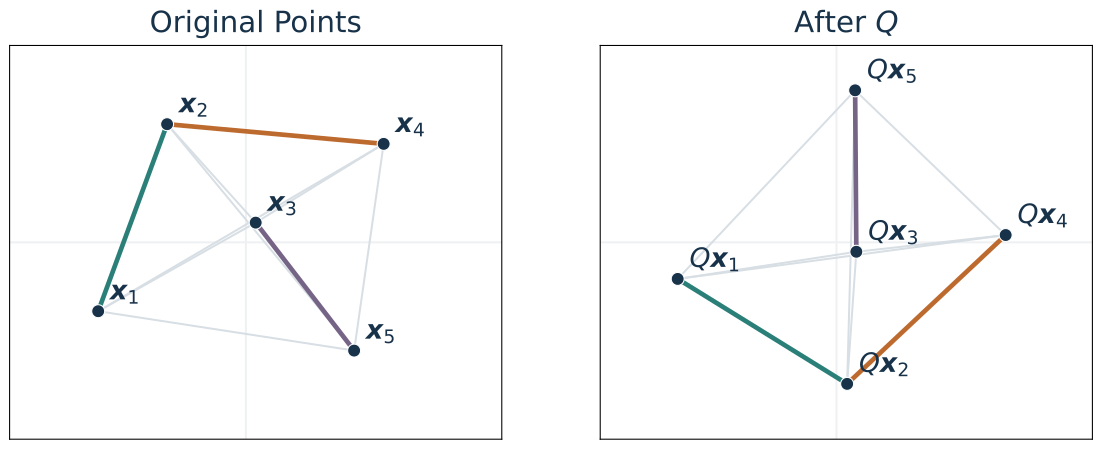
Orthogonality preserves all pairwise Euclidean distances

For any \(\boldsymbol{x}_i,\boldsymbol{x}_j\in\mathbb{R}^{d}\) and orthogonal \(Q\):

\(\displaystyle \lVert Q\boldsymbol{x}_i-Q\boldsymbol{x}_j\rVert_2\)

\(=\)

\(\displaystyle \lVert Q(\boldsymbol{x}_i-\boldsymbol{x}_j)\rVert_2\)

(Distributivity)

\(\,\)

\(=\)

\(\displaystyle \sqrt{(\boldsymbol{x}_i-\boldsymbol{x}_j)^TQ^TQ(\boldsymbol{x}_i-\boldsymbol{x}_j)}\)

(Euclidean norm)

\(\,\)

\(=\)

\(\displaystyle \sqrt{(\boldsymbol{x}_i-\boldsymbol{x}_j)^T(\boldsymbol{x}_i-\boldsymbol{x}_j)}\)

(\(Q^TQ=I\))

\(\,\)

\(=\)

\(\displaystyle \lVert\boldsymbol{x}_i-\boldsymbol{x}_j\rVert_2\)

(Euclidean norm)

This is the first formal proof in the redesigned technical sequence. Reveal one line per click. Read the matrix product in the second equality carefully and pause at Q^TQ=I, which carries the entire preservation claim.

Diagonal and orthogonal matrices have simple interpretations

Diagonal: Scale Each Coordinate

\[ D=\operatorname{diag}(d_1,\ldots,d_d), \qquad y_j=d_jx_j \]

• Each coordinate undergoes ordinary scalar multiplication.
• The sign keeps or reverses its direction.
• The magnitude stretches or shrinks it; zero collapses it.

Orthogonal: Rotate or Reflect

\[ \boldsymbol{y}=Q\boldsymbol{x}, \qquad Q^TQ=I \]

• Rotate, reflect, or combine both about the origin.
• Keep lengths, angles, and pairwise distances unchanged.
• Change orientation without stretching or shrinking.

Recap the diagonal examples from Friday and the orthogonal example just proved. In higher dimensions, rotations can occur in multiple planes and reflections are through subspaces through the origin. No translation occurs: the origin stays fixed. The identity is the case that leaves the orientation unchanged. For the diagonal case, x_j is a scalar coordinate, so each rule is the familiar one-dimensional multiplication rule.

In 1D, sign and magnitude explain what multiplication does

One Dimension

For \(a\ne0\):

\[ y=ax=\underbrace{\operatorname{sign}(a)}_{\text{keep or reverse}} \quad\underbrace{|a|}_{\text{scale}}\,x \]

For example, \(-3x=(-1)(3)x\):

• \(3\): stretch by a factor of three.
• \(-1\): reverse direction.

Higher Dimensions

\[ \boldsymbol{y}=A\boldsymbol{x} \]

We know how to calculate the output. But for an arbitrary matrix:

• Which directions change, and how?
• How much does each direction stretch or shrink?
• Can any direction collapse entirely?

Can we decompose any \(A\) into rotations or reflections and independent scalings so that we can understand and analyze what it does?

Knowing the row-by-column recipe does not yet give an intuitive description of an arbitrary linear operator. In 1D, sign and magnitude separate two familiar roles; ask for an analogous separation in higher dimensions. If a = 0, every input collapses to zero, so no direction choice matters. SVD will provide two orthogonal factors and nonnegative scalings, not an entrywise matrix-sign rule. The two orientation changes allow input and output directions to differ.

SVD separates every linear transformation into three understandable steps

Let \(U\Sigma V^T\) be the singular value decomposition (SVD) of \(A\), i.e., \(A=U\Sigma V^T\).

\(U\) and \(V\) are orthogonal; \(\Sigma\) is diagonal (possibly rectangular).

\[ \boldsymbol{y}=A\boldsymbol{x} =U\Sigma V^T\boldsymbol{x} =U\bigl(\Sigma(V^T\boldsymbol{x})\bigr) \]

Read the equation from right to left. The asymmetric shape makes each orientation change visible. The two orthogonal factors play the orientation role that the sign played in 1D; Sigma contains nonnegative magnitudes. Sigma is the only stage that changes Euclidean distances. Read each stage as a familiar operation before returning to the compact factorization.

Each SVD factor has a precise shape and role

For \(A\in\mathbb{R}^{m\times d}\), the full SVD is:

\[ \underbrace{A}_{m\times d} = \underbrace{U}_{m\times m} \quad\underbrace{\Sigma}_{m\times d} \quad\underbrace{V^T}_{d\times d} \]

Factor	Mathematical Property	What It Does
\(U\)	Square and orthogonal: \(U^TU=I_m\)	Rotates or reflects in the output space.
\(\Sigma\)	Same shape as \(A\); \(\Sigma_{ij}=0\) whenever \(i\ne j\)	Scales directions; zero scalings can collapse them.
\(V^T\)	Square and orthogonal: \(V^TV=VV^T=I_d\)	Rotates or reflects in the input space.

\(\Sigma\) is rectangular diagonal: only \(\Sigma_{ii}=\sigma_i\ge0\) may be nonzero, for \(i=1,\ldots,\min(m,d)\).

Read all four shapes aloud and check the inner dimensions of the product. U and V are square orthogonal matrices in the full SVD; their transposes are also orthogonal. The subscript on each identity gives its size. Sigma has exactly the same number of rows and columns as A. Rectangular diagonal means only entries with matching row and column indices may be nonzero; any extra rows or columns are entirely zero. Economy-size SVD conventions remain deferred.

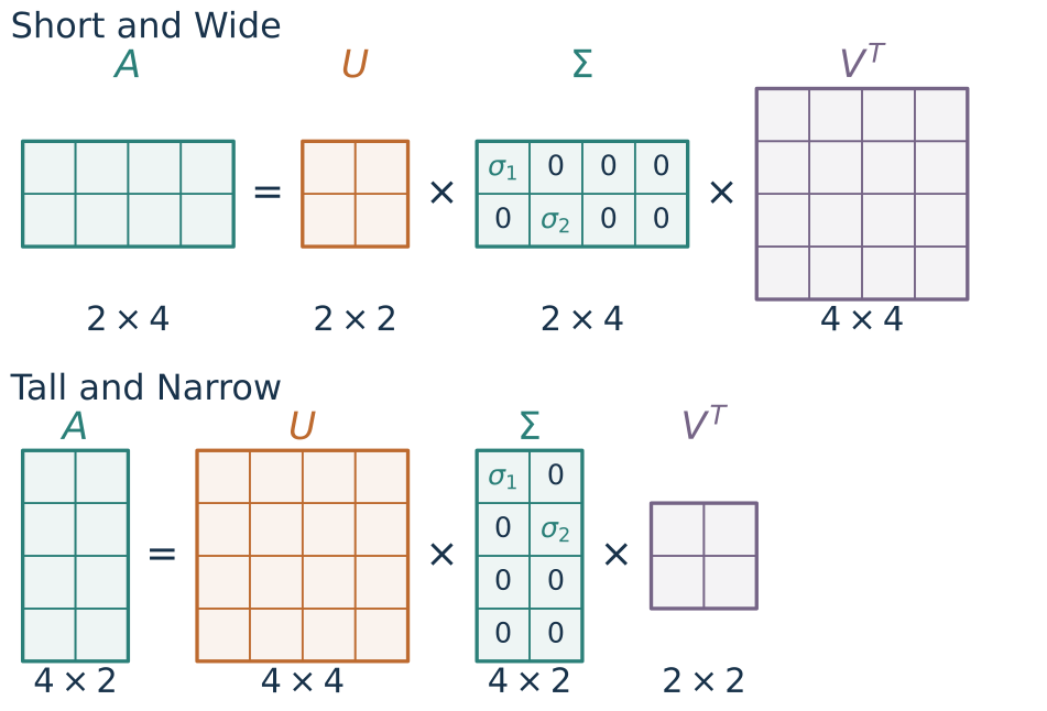
\(A\) and \(\Sigma\) share a shape; the orthogonal factors are square

\(U\): square, sized by the rows of \(A\).

\(V^T\): square, sized by the columns of \(A\).

These are dimension diagrams, not numerical entries of a particular matrix. Each cell represents one entry. Both examples use the full SVD. The wide case has zero columns after Sigma’s two diagonal positions; the tall case has zero rows below them. Point out that U uses the output dimension m while V uses the input dimension d. Ask students to check the matrix products from right to left.

Singular values tell us how much each direction scales

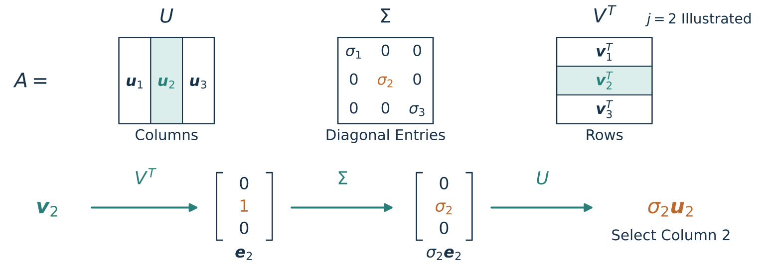
\[ V^T\boldsymbol{v}_j=\boldsymbol{e}_j \quad\Longrightarrow\quad A\boldsymbol{v}_j=U(\Sigma\boldsymbol{e}_j)=\sigma_j\boldsymbol{u}_j, \qquad j\le\min(m,d). \]

The diagram uses a square 3 by 3 example and j=2; the equation applies to full rectangular SVD with j <= min(m,d). Rows of V transpose compute v_i transpose v_j, which is 1 for i=j and 0 otherwise. Sigma produces sigma_j times the output-space basis vector; U selects its jth column. In rectangular cases the input and output basis vectors have lengths d and m respectively. Singular values above one stretch, below one shrink, and zero collapses a direction.

The largest singular value gives the maximum stretching

Order the singular values: \(\sigma_1\ge\sigma_2\ge\cdots\ge0\).

\[ \|A\boldsymbol{x}\|_2\le\sigma_1\|\boldsymbol{x}\|_2, \qquad \|A\|_2:=\max_{\|\boldsymbol{x}\|_2=1}\|A\boldsymbol{x}\|_2=\sigma_1. \]

• \(V^T\) and \(U\) preserve lengths.
• Each coordinate scaling in \(\Sigma\) is at most \(\sigma_1\).
• The input \(\boldsymbol{v}_1\) attains the largest scaling.

Introduce the operator or spectral norm as a maximum amplification, distinguishing it from the Euclidean norm of a vector. For a zero matrix the maximum is zero. The same bound applies to pairwise differences by linearity. Do not introduce condition numbers or optimization here.

Rank counts the independent directions that survive

\[ \operatorname{rank}(A)=\#\{j:\sigma_j>0\}\le\min(m,d) \]

For example:

\[ \Sigma=\begin{bmatrix}3&0&0\\0&1&0\\0&0&0\end{bmatrix} \qquad\Longrightarrow\qquad \operatorname{rank}(A)=2 \]

• Two independent input directions produce nonzero output directions.
• The third input direction disappears: \(A\boldsymbol{v}_3=\boldsymbol{0}\).
• Rotations and reflections change which directions these are, but not the rank.

Define rank as the dimension of the possible output space, then use the SVD to count that dimension. Rank belongs to an operator; do not confuse it with the number of distinct points in one finite dataset. Numerical near-zero thresholds come later; this slide concerns exact mathematical rank.

A null direction makes different inputs indistinguishable

The null space contains all directions that map to zero:

\[ \operatorname{null}(A)=\{\boldsymbol{h}:A\boldsymbol{h}=\boldsymbol{0}\}. \]

For any nonzero \(\boldsymbol{h}\in\operatorname{null}(A)\):

\(\displaystyle A(\boldsymbol{x}+\boldsymbol{h})\)

\(=\)

\(\displaystyle A\boldsymbol{x}+A\boldsymbol{h}\)

(Distributivity)

\(\,\)

\(=\)

\(\displaystyle A\boldsymbol{x}\)

(Null direction)

The ambiguity is structural: any amount of movement along a null direction is invisible to the operator. It is not caused by a poor numerical algorithm.

A square operator is invertible when no direction collapses

In 1D, \(y=ax\) can be undone by \(x=y/a\) exactly when \(a\ne0\).

For square \(A=U\Sigma V^T\in\mathbb{R}^{d\times d}\):

\[ \text{all }\sigma_j>0 \quad\Longrightarrow\quad A^{-1}=V\Sigma^{-1}U^T, \qquad \Sigma^{-1}=\operatorname{diag}(1/\sigma_1,\ldots,1/\sigma_d). \]

\(\displaystyle A^{-1}A\)

\(=\)

\(\displaystyle (V\Sigma^{-1}U^T)(U\Sigma V^T)\)

(Substitute)

\(\,\)

\(=\)

\(\displaystyle V\Sigma^{-1}\Sigma V^T\)

(\(U^TU=I_d\))

\(\,\)

\(=\)

\(\displaystyle VV^T\)

(\(\Sigma^{-1}\Sigma=I_d\))

\(\,\)

\(=\)

\(\displaystyle I_d\)

(\(VV^T=I_d\))

The displayed computation verifies the proposed inverse. For a square matrix, a left inverse is also its inverse. An orthogonal factor is always invertible: Q inverse is Q transpose. Any failure of a square SVD to be invertible lies in a zero singular value. An invertible transformation may still distort distances; invertibility is not orthogonality.

Recovery depends on preserving every input direction

\(\boldsymbol{y}=A\boldsymbol{x}\) maps \(d\) input coordinates to \(m\) output coordinates.

Recovering every \(\boldsymbol{x}\in\mathbb{R}^d\) requires \(\operatorname{rank}(A)=d\).

The blocks show dimensions, not entries of specific matrices. Full column rank means no nonzero input is mapped to zero. More outputs permit this condition but do not guarantee it. A map with m<d can still distinguish a particular finite dataset or preserve a restricted subspace; the claim here concerns every input.

The pseudoinverse undoes every nonzero scaling

For any \(A=U\Sigma V^T\in\mathbb{R}^{m\times d}\), define:

\[ \underbrace{A^\dagger}_{d\times m} =\underbrace{V}_{d\times d}\underbrace{\Sigma^\dagger}_{d\times m}\underbrace{U^T}_{m\times m}. \]

\(\Sigma^\dagger\) has the transposed shape of \(\Sigma\), with zero off-diagonal entries:

\[ (\Sigma^\dagger)_{jj}= \begin{cases} 1/\sigma_j, & \sigma_j>0,\\ 0, & \sigma_j=0. \end{cases} \]

• Reverse the output reorientation, undo nonzero scalings, then reorient back.
• A zero scaling destroyed information; leaving it zero cannot restore it.
• The Moore–Penrose pseudoinverse exists even when \(A\) has no inverse.

For j up to min(m,d), reciprocate positive singular values and keep zero values zero; every other entry is zero. This defines the unique Moore–Penrose inverse regardless of nonuniqueness in SVD factors. It exists for every real matrix, including the zero matrix. If A is square and invertible, this is exactly the inverse formula just proved. Numerical thresholds for tiny singular values are a separate numerical-computation issue. No four-identity axiom list is needed for the conceptual role here. It is useful later for least squares, but not a prerequisite for deriving the PCA reconstruction objective.

The pseudoinverse recovers inputs exactly when no input direction is lost

For \(\boldsymbol{y}=A\boldsymbol{x}\), recovery of every input means:

\[ \widehat{\boldsymbol{x}}=A^\dagger\boldsymbol{y}=\boldsymbol{x} \ \text{for all }\boldsymbol{x}\in\mathbb{R}^d \quad\Longleftrightarrow\quad A^\dagger A=I_d. \]

Let \(r=\operatorname{rank}(A)\) and \(V_r=[\boldsymbol{v}_1\;\cdots\;\boldsymbol{v}_r]\) contain its surviving input directions.

\(\displaystyle A^\dagger A\)

\(=\)

\(\displaystyle V\Sigma^\dagger U^TU\Sigma V^T\)

(Substitute)

\(\,\)

\(=\)

\(\displaystyle V(\Sigma^\dagger\Sigma)V^T\)

(\(U^TU=I_m\))

\(\,\)

\(=\)

\(\displaystyle V_rV_r^T\)

(Keep nonzero directions)

\(\Sigma^\dagger\Sigma\) has \(r\) diagonal ones and \(d-r\) zeros. Thus \(A^\dagger A=I_d\) exactly when \(r=d\): full column rank, requiring \(m\ge d\).

Order singular values with positive values first. V_r V_r transpose keeps the component in the surviving input subspace and removes null-space components. If r=0, interpret this as the zero matrix. For a particular input outside this subspace, the lost component is unidentifiable from y. A reconstruction algorithm cannot recover every input from the same output when multiple inputs share it. More output coordinates only permit full column rank; they do not ensure it. The pseudoinverse exists regardless of whether this exact-recovery condition holds.

A restricted input subspace can be recovered exactly

Inputs: \(\boldsymbol{x}=t\boldsymbol{u}\in\mathbb{R}^2\), \(\|\boldsymbol{u}\|_2=1\). Encoder: \(A=\boldsymbol{v}^T\), with \(\alpha=\boldsymbol{v}^T\boldsymbol{u}\ne0\).

Decode with \(B=\boldsymbol{u}/\alpha\): knowing the line lets us undo its nonzero scaling.

\[ \widehat{\boldsymbol{x}}=By=\frac{\boldsymbol{u}}{\alpha}(\alpha t)=t\boldsymbol{u}=\boldsymbol{x}. \]

If \(\boldsymbol{v}=\boldsymbol{u}\), then \(\alpha=1\), \(y=t\), and \(B=A^\dagger=\boldsymbol{u}\). In general, \(B\ne A^\dagger\).

Ambient dimension is 2; intrinsic dimension is 1. Every nonperpendicular encoder direction v works: v^T u != 0 ensures distinct t give distinct outputs. If v is perpendicular to u, every point on the line maps to zero and recovery is impossible. The figure uses u=(0.8,0.6), v=(1,0), so alpha=0.8. B is the inverse of A restricted to the known line, not generally the Moore-Penrose pseudoinverse of A on the ambient space. For A=v^T, A^dagger=v/(vT v) selects the minimum-norm ambient solution, which generally lies along v rather than along the known input line u. BA acts as the identity on S even though BA != I_2. When v=u is unit length, B=A^dagger=u and y=t. More generally, recovery on a known subspace S is possible iff S intersects null(A) only at zero. A line through the origin is a linear subspace and a simple embedded manifold; shifted lines require an offset, and curved manifolds need not admit one global linear coordinate.

Read what an operator does from its singular values

A sensor-processing system uses \(A=U\operatorname{diag}(4,1,0)V^T\).

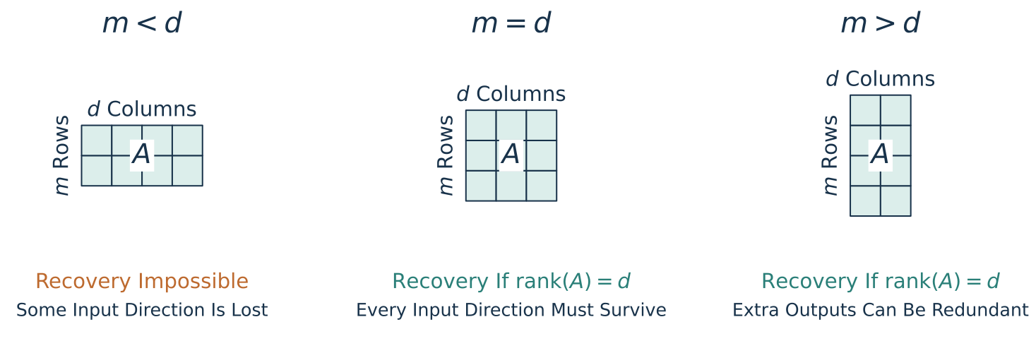
Can you recover every sensor input? What is the largest possible stretching factor? Could this operator preserve every pairwise distance? Explain which input direction is invisible to the system.

Rank \(2\); recovery is impossible in general; maximum scaling is \(4\). The direction \(\boldsymbol{v}_3\) disappears. All distances cannot be preserved.

Pairs, 3–4 minutes. Students must connect each claim to a singular value, not just name a property. Ask whether observing distinct outputs for a small test sample would overturn the recovery conclusion: it would not.

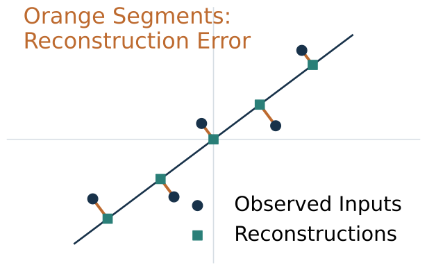
Data near a subspace can have small reconstruction error

What if the inputs are close to a line, but do not lie exactly on it?

\[ y=\boldsymbol{u}^T\boldsymbol{x},\qquad \widehat{\boldsymbol{x}}=\boldsymbol{u}y,\qquad \text{error}=\|\boldsymbol{x}-\widehat{\boldsymbol{x}}\|_2^2. \]

Which direction minimizes total reconstruction error?

The exact line case has zero error. Near the line, each residual is perpendicular to the retained direction and is discarded by the encoder. Small residuals mean approximate recovery, not exact inversion. Here the line passes through the origin; the next topic centers observations before choosing a subspace. The figure is illustrative synthetic data. Do not claim that this displayed line is already the optimal PCA line; selecting that line is the coming problem.