Reconstruction and Principal Component Analysis

David I. Inouye

Dynamic Content · Last Updated: September 11, 2026

This topic formalizes dimensionality reduction through reconstruction, then derives PCA. It assumes the preceding topic’s SVD, rank, and recoverability results. Topic boundaries are conceptual; class meetings may stop within either topic.

A useful reduction should reconstruct the observed data well

Return to the cells described by many measured features.

• Fewer coordinates cannot preserve every possible input exactly.
• The observed data may nevertheless lie near a lower-dimensional subspace.
• We will judge a representation by how well it reconstructs those observations.

What reconstruction error are we willing to accept in exchange for fewer features?

Four steps lead to the PCA formulation

We will turn “reconstruct the data well” into a problem involving one matrix.

1. Define what a good reconstruction means — Next

Choose a representation size and measure reconstruction error.

2. Choose a convenient decoder basis.

An orthonormal basis can represent the same reconstruction subspace.

3. Find the best encoder for that decoder.

The closest point in the subspace determines the coordinates.

4. Formulate the subspace choice.

Combine these results into the PCA optimization problem.

Centering separates the mean from variation

For notation simplicity, we now call the raw data \(\widetilde X\) and the centered data \(X\).

\[ \boldsymbol{\mu}=\frac1n\sum_{i=1}^n\widetilde{\boldsymbol{x}}_i, \qquad X=\widetilde X-\boldsymbol{1}_n\boldsymbol{\mu}^T. \]

• Each row is \(\boldsymbol{x}_i^T=(\widetilde{\boldsymbol{x}}_i-\boldsymbol{\mu})^T\).
• Every feature column of \(X\) has mean zero.
• From here on, \(X\) and \(\boldsymbol{x}_i\) always denote centered data.

Add the mean back to reconstruct raw measurements: \(\widehat{\widetilde{\boldsymbol{x}}}_i=\boldsymbol{\mu}+\widehat{\boldsymbol{x}}_i\).

The preceding topic used X for general data. Announce this local notation change explicitly: tilde marks raw observations; unadorned symbols mean centered data. Both matrices have n rows and d columns. Define the all-ones vector 1_n and show its product with mu transpose repeats the mean row. Centering does not standardize different measurement units. In the cell example, preprocessing choices still determine what Euclidean error means.

A linear encoder and decoder make reconstruction explicit

For one centered observation, use the same operator convention as \(\boldsymbol{y}=A\boldsymbol{x}\):

\[ \boldsymbol{z}_i=\underbrace{E}_{k\times d}\boldsymbol{x}_i, \qquad \widehat{\boldsymbol{x}}_i=\underbrace{D}_{d\times k}\boldsymbol{z}_i. \]

Stacking observations as rows gives:

\[ \underbrace{Z}_{n\times k} =\underbrace{X}_{n\times d}\underbrace{E^T}_{d\times k}, \qquad \underbrace{\widehat X}_{n\times d} =\underbrace{Z}_{n\times k}\underbrace{D^T}_{k\times d}. \]

The batch reconstruction is \(\widehat X=XE^TD^T\), with rank at most \(k\).

D here is a general decoder, not the diagonal matrix from the earlier operator examples. The rank-at-most-k requirement comes from passing through k features. Do not assume D equals E transpose at this stage.

Reconstruction error formalizes one meaning of preservation

Choose a linear encoder and decoder to minimize squared reconstruction error:

\[ \min_{E,D}\|X-XE^TD^T\|_F^2. \]

The Frobenius norm measures the error across every entry:

\[ \|M\|_F^2=\sum_{i,j}M_{ij}^2, \qquad \|X-\widehat X\|_F^2 =\sum_{i=1}^n\|\boldsymbol{x}_i-\widehat{\boldsymbol{x}}_i\|_2^2. \]

Bridge the new matrix norm by summing the familiar vector squared error across observations. The objective treats measured coordinates according to their scale; it does not automatically encode biological meaning or downstream usefulness.

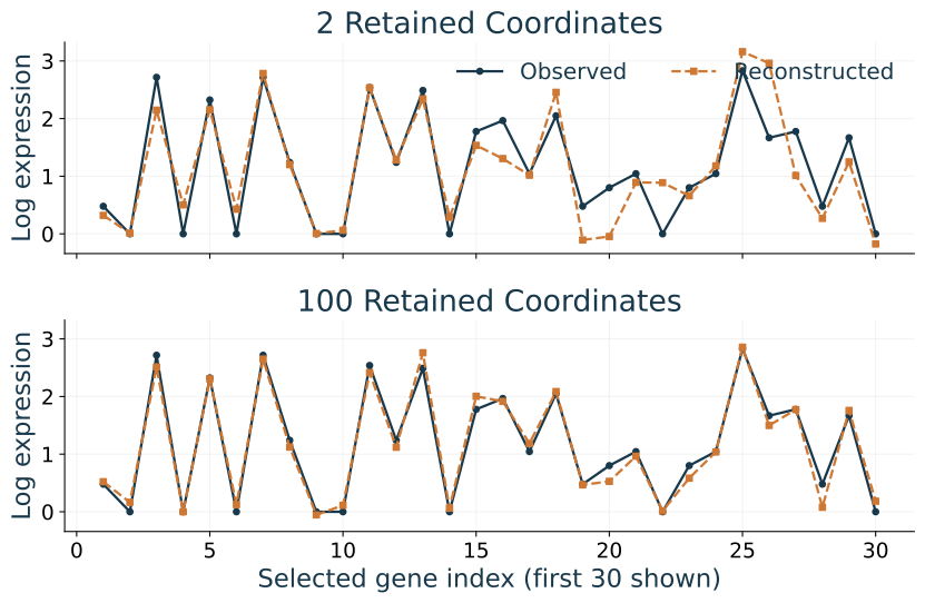
Four steps lead to the PCA formulation

We have an error measure. Now consider which reconstructions the decoder can produce.

1. Define what a good reconstruction means — Established

Choose a representation size and measure reconstruction error.

2. Choose a convenient decoder basis — Next

An orthonormal basis can represent the same reconstruction subspace.

3. Find the best encoder for that decoder.

The closest point in the subspace determines the coordinates.

4. Formulate the subspace choice.

Combine these results into the PCA optimization problem.

Matrix–vector multiplication combines the matrix’s columns

For a \(3\times2\) decoder, the familiar row dot products can be regrouped by column:

\[ \begin{bmatrix}d_{11}&d_{12}\\d_{21}&d_{22}\\d_{31}&d_{32}\end{bmatrix} \begin{bmatrix}z_1\\z_2\end{bmatrix} = \underbrace{\begin{bmatrix}d_{11}z_1+d_{12}z_2\\d_{21}z_1+d_{22}z_2\\d_{31}z_1+d_{32}z_2\end{bmatrix}}_{\text{one dot product per row}} = z_1\underbrace{\begin{bmatrix}d_{11}\\d_{21}\\d_{31}\end{bmatrix}}_{\boldsymbol{d}_1} +z_2\underbrace{\begin{bmatrix}d_{12}\\d_{22}\\d_{32}\end{bmatrix}}_{\boldsymbol{d}_2}. \]

For any number of columns: \(\widehat{\boldsymbol{x}}=D\boldsymbol{z}=\sum_{j=1}^k z_j\boldsymbol{d}_j\).

• Let \(\boldsymbol{z}\) be arbitrary for now. Every reconstruction lies in \(\mathcal{S}=\operatorname{span}\{\boldsymbol{d}_1,\ldots,\boldsymbol{d}_k\}\).
• First choose how \(D\) describes that subspace; then choose the best coordinates.

Point to each entry in the middle vector, then collect all z1 terms into the first column and all z2 terms into the second. These are two interpretations of the same multiplication. Column vectors d_j live in the original d-dimensional space. No encoder has been chosen: z is any vector in R^k. The decoder limits where a reconstruction can lie regardless of how z is produced. All inputs in this topic are centered; observations are stacked as rows only in batch formulas.

Scaling a decoder direction only changes its coordinates

A line can use a unit vector \(\boldsymbol{u}\) or the scaled vector \(3\boldsymbol{u}\).

\[ \underbrace{\boldsymbol{u}}_{\text{unit basis}}\underbrace{t}_{\text{coordinate}} = \underbrace{(3\boldsymbol{u})}_{\text{scaled basis}}\underbrace{(t/3)}_{\text{adjusted coordinate}}. \]

Both describe the same point on the same line.

• A nonzero column can be normalized if we rescale its coordinate to compensate.
• Unit columns remove an arbitrary scale choice; no reconstruction is lost.
• Next: can we choose perpendicular columns while keeping the same subspace?

This is a parameterization choice, not a claim that unit vectors reconstruct better than scaled ones. For column d_j=c_j w_j with c_j=norm(d_j)>0, d_j z_j=w_j(c_j z_j). Zero columns contribute nothing. Normalization alone does not make different columns perpendicular; address that separately next.

Perpendicular unit directions can describe the same subspace

Both unit-vector pairs span the plane: either represents every \(\boldsymbol{x}=[x_1,x_2]^T\).

For \(\boldsymbol{b}_1=[1,0]^T\), \(\boldsymbol{b}_2=[1,1]^T/\sqrt2\):

\[ \boldsymbol{x}=(x_1-x_2)\boldsymbol{b}_1+\sqrt2\,x_2\boldsymbol{b}_2. \]

For \(\boldsymbol{w}_1=[1,0]^T\), \(\boldsymbol{w}_2=[0,1]^T\):

\[ \boldsymbol{x}=(\boldsymbol{w}_1^T\boldsymbol{x})\boldsymbol{w}_1 +(\boldsymbol{w}_2^T\boldsymbol{x})\boldsymbol{w}_2. \]

Same plane; simpler coordinates: an orthonormal basis gives each coefficient by a dot product.

The retained plane is drawn face-on. Both panels show the same point [2,1]^T. Left: b1=[1,0]^T, b2=[1,1]^T/sqrt(2), so x=b1+sqrt(2)b2. Right: x=2w1+w2. For any x=[x1,x2]^T, expanding (x1-x2)b1+sqrt(2)x2 b2 gives [x1,x2]^T. Thus both independent unit pairs span the entire plane, not only this example. For a skew unit basis, b1^T x=z1+(b1^T b2)z2; b2^T x=(b2^T b1)z1+z2. Individual dot products mix coefficients. Dividing by each basis vector’s squared norm does not undo that mixing. For an orthogonal non-unit basis, z_j=(b_j^T x)/(b_j^T b_j) does work; orthonormality also removes the denominator. Every subspace admits an orthonormal basis. It is not unique; changing the basis changes coordinates, not reconstruction possibilities. The next slide formalizes how to absorb the coordinate change into the encoder.

QR lets us choose an orthonormal decoder without changing reconstruction

Start with any encoder \(E_0\in\mathbb{R}^{k\times d}\) and decoder \(D_0\in\mathbb{R}^{d\times k}\), where \(k\le d\). Suppose \(D_0\) does not have orthonormal columns.

The thin QR decomposition writes \(D_0=WR\): \(W^TW=I_k\) and \(R\) is upper triangular. Here \(W\in\mathbb{R}^{d\times k}\) and \(R\in\mathbb{R}^{k\times k}\).

Can we choose \(D=W\) and a new \(E\) to keep every reconstruction the same?

\(\displaystyle D_0E_0\boldsymbol{x}\)

\(=\)

\(\displaystyle (WR)E_0\boldsymbol{x}\)

(QR of the original decoder)

\(\,\)

\(=\)

\(\displaystyle W(RE_0)\boldsymbol{x}\)

(Regroup the factors)

\(\,\)

\(=\)

\(\displaystyle DE\boldsymbol{x}\)

(Choose \(D=W\), \(E=RE_0\))

Same reconstruction for every input: an orthonormal decoder is without loss of generality. Next, fix \(D=W\) and find its best encoder.

Introduce both original operators before factoring the decoder. QR is another standard matrix decomposition, introduced here because it solves a specific problem. The factor usually named Q is called W to match our subspace notation. In thin QR for d by k with k<=d, W has k orthonormal columns and R is k by k upper triangular (entries below the diagonal are zero). If D0 has full column rank, W is a basis of exactly its column span and R is invertible. Thin QR also exists for deficient rank: W spans a k-dimensional space containing the decoder span, and R is singular. We never invert R, so the reconstruction identity holds in either case. For a general rectangular matrix, full QR uses a square orthogonal Q and an upper-trapezoidal R; avoid saying every rectangular R is square triangular. We do not need to teach the QR algorithm here. Triangularity is a property of this standard factorization, not needed for the regrouping. The new encoder RE0 remains arbitrary; its optimal choice W^T is derived next. With row-stacked inputs the identity is X E0^T D0^T = X E^T D^T.

Four steps lead to the PCA formulation

We may choose an orthonormal decoder without changing what we can reconstruct.

1. Define what a good reconstruction means — Established

Choose a representation size and measure reconstruction error.

2. Choose a convenient decoder basis — Established

An orthonormal basis can represent the same reconstruction subspace.

3. Find the best encoder for that decoder — Next

The closest point in the subspace determines the coordinates.

4. Formulate the subspace choice.

Combine these results into the PCA optimization problem.

In 2D, the perpendicular foot is the best reconstruction

Any unit \(\boldsymbol{u}\) works. Illustrate with \(\boldsymbol{u}=[1,0]^T\), so \(\boldsymbol{q}=z\boldsymbol{u}=[z,0]^T\).

\(\displaystyle \|\boldsymbol{x}-\boldsymbol{q}\|_2^2\)

\(=\)

\(\displaystyle (x_1-q_1)^2+(x_2-q_2)^2\)

(Squared distance)

\(\,\)

\(=\)

\(\displaystyle (2-z)^2+(2-0)^2\)

(Substitute coordinates)

\(\,\)

\(=\)

\(\displaystyle (2-z)^2+4\)

(Simplify)

Choose \(z=2\): the horizontal error is zero; the height remains.

For any unit u, the optimal coordinate is z=u^T x and the reconstruction is u u^T x. Rotating the line and input together preserves distances, so the horizontal example illustrates the general result. The coordinate calculation uses u=[1,0]^T only to keep its entries simple. The orange arrow is the decoder column u, with unit length measured from the explicitly marked origin. All q candidates are points, not basis arrows. The labels q_a,q_b,q_c distinguish candidate points; q_1,q_2 in the norm definition are the scalar coordinates of an arbitrary q. For candidate coordinates z=1,2,3, squared errors are 5,4,5 respectively. Both moving before and after the perpendicular foot add horizontal squared error. The norm formula is the sum of squares of coordinate differences: no geometric error decomposition is assumed here. The fixed second coordinate of every candidate is zero, so no choice of z can remove the vertical difference 2. The plane example next generalizes this coordinate calculation via Pythagoras.

In 3D, moving within the plane cannot remove the height

Fix \(D=W\) with two orthonormal columns spanning this plane. Which point should we reconstruct?

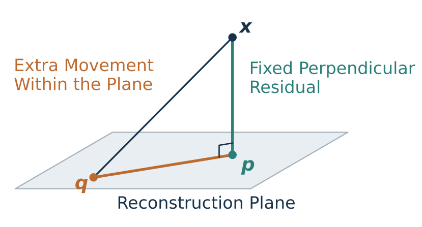
\[ \|\boldsymbol{x}-\boldsymbol{q}\|_2^2 =\underbrace{\|\boldsymbol{x}-\boldsymbol{p}\|_2^2}_{\text{fixed perpendicular error}} +\underbrace{\|\boldsymbol{p}-\boldsymbol{q}\|_2^2}_{\text{extra error within the plane}}. \]

Choose \(\boldsymbol{q}=\boldsymbol{p}\). Moving in either plane direction only adds error.

This is a 3D plane viewed obliquely; the right-angle marker is constructed in 3D and projected with the plane. The residual is perpendicular to every in-plane direction, not only the displayed orange leg. Any candidate q gives a right triangle in the slice through x,p,q. This is why the line intuition generalizes.

A dot product gives the length along a unit direction

Recall \(\boldsymbol{u}^T\boldsymbol{x}=\|\boldsymbol{u}\|_2\|\boldsymbol{x}\|_2\cos\theta\). Here \(\|\boldsymbol{u}\|_2=1\).

\(\displaystyle a\)

\(=\)

\(\displaystyle \text{hypotenuse}\,\frac{\text{adjacent}}{\text{hypotenuse}}\)

(\(a\) = adjacent length)

\(\,\)

\(=\)

\(\displaystyle \|\boldsymbol{x}\|_2\cos\theta\)

(Definition of cosine)

\(\,\)

\(=\)

\(\displaystyle \boldsymbol{u}^T\boldsymbol{x}\)

(Dot product; \(\|\boldsymbol{u}\|_2=1\))

The foot is \((\boldsymbol{u}^T\boldsymbol{x})\boldsymbol{u}\). This works in any dimension.

Use the standard dot-product identity as a recalled fact, not a new proof. The adjacent length is the hypotenuse times the adjacent/hypotenuse ratio; that ratio is cos(theta). The recalled identity then gives u^T x for unit u. Here x=[2,2]^T, u=[1,0]^T, norm(x)=sqrt(8), theta=pi/4, and a=2. The geometry applies to any two vectors u and x in any dimension: their span has dimension at most two. Normalize a nonzero u first; without normalization, the signed length is u^T x / norm(u), and the foot is u(u^T x)/(u^T u). In general a is signed: an obtuse angle places the foot on the opposite side of the origin. If x=0, the coefficient is zero without defining theta.

Coordinates along the basis directions locate the point in the plane

For a plane with orthonormal basis \(\boldsymbol{w}_1,\boldsymbol{w}_2\), read the two signed lengths:

\[ a_1=\boldsymbol{w}_1^T\boldsymbol{x},\qquad a_2=\boldsymbol{w}_2^T\boldsymbol{x}. \]

Combine the corresponding moves within the plane:

\[ \boldsymbol{p}=a_1\boldsymbol{w}_1+a_2\boldsymbol{w}_2 =\begin{bmatrix}\boldsymbol{w}_1&\boldsymbol{w}_2\end{bmatrix} \begin{bmatrix}a_1\\a_2\end{bmatrix}=W\boldsymbol{a}. \]

• Perpendicular basis directions let us read each coordinate independently.
• For \(k\) orthonormal directions, the same construction gives \(\boldsymbol{a}=W^T\boldsymbol{x}\) and \(\boldsymbol{p}=W\boldsymbol{a}\).

Next, verify the geometry algebraically: is \(\boldsymbol{x}-\boldsymbol{p}\) perpendicular to every decoder direction?

Do not sum distances; sum the scaled basis vectors. Each scalar a_j measures a signed displacement along w_j. A move along w2 leaves the w1 coordinate unchanged, and vice versa, because w1^T w2=0. Thus p has the same two in-plane components as x. For x=[2,1,2]^T and the xy plane, a=[2,1]^T and p=[2,1,0]^T. Distinguish p, the foot on the full plane, from a1 w1, the foot on just one line. The next slide verifies the perpendicular residual rather than assuming that stacking these coordinates automatically proves optimality. The later error split proves p is the unique closest reconstruction.

The residual is perpendicular to every decoder direction

Fix \(D=W\), with \(W^TW=I_k\). For one centered input, define:

\[ \boldsymbol{a}=W^T\boldsymbol{x},\qquad \boldsymbol{p}=W\boldsymbol{a},\qquad \boldsymbol{r}=\boldsymbol{x}-\boldsymbol{p}. \]

The point \(\boldsymbol{p}\) lies in the decoder’s subspace. Check its residual:

\(\displaystyle W^T\boldsymbol{r}\)

\(=\)

\(\displaystyle W^T(\boldsymbol{x}-W\boldsymbol{a})\)

(Substitute the residual)

\(\displaystyle \,\)

\(=\)

\(\displaystyle W^T\boldsymbol{x}-W^TW\boldsymbol{a}\)

(Distribute)

\(\displaystyle \,\)

\(=\)

\(\displaystyle \boldsymbol{a}-\boldsymbol{a}=\boldsymbol{0}\)

(\(\boldsymbol{a}=W^T\boldsymbol{x}\) and \(W^TW=I_k\))

Each entry is \(\boldsymbol{w}_j^T\boldsymbol{r}=0\): the residual is perpendicular to every basis direction.

a denotes candidate optimal coordinates, not assumed optimal yet. We construct p and verify it is the perpendicular foot before claiming it minimizes error. The residual r depends on x and the chosen subspace, not on the later arbitrary coordinate z. The equalities generalize the fixed height in both illustrations.

Every reconstruction error has two perpendicular parts

For any coordinates \(\boldsymbol{z}\), the decoder returns \(W\boldsymbol{z}\). Insert the perpendicular foot \(\boldsymbol{p}=W\boldsymbol{a}\):

\(\displaystyle \boldsymbol{x}-W\boldsymbol{z}\)

\(=\)

\(\displaystyle (\boldsymbol{x}-\boldsymbol{p})+(\boldsymbol{p}-W\boldsymbol{z})\)

(Add and subtract the same point)

\(\displaystyle \,\)

\(=\)

\(\displaystyle \boldsymbol{r}+(W\boldsymbol{a}-W\boldsymbol{z})\)

(Substitute the two parts)

\(\displaystyle \,\)

\(=\)

\(\displaystyle \boldsymbol{r}+W(\boldsymbol{a}-\boldsymbol{z})\)

(Factor out the decoder)

• \(\boldsymbol{r}\) is the fixed perpendicular part, outside the subspace.
• \(W(\boldsymbol{a}-\boldsymbol{z})\) is the adjustable part, inside the subspace.

Changing \(\boldsymbol{z}\) moves only within the subspace, so it cannot cancel \(\boldsymbol{r}\).

Connect the two terms explicitly to the teal and orange legs in both figures. Their inner product is r^T W(a-z)=(W^T r)^T(a-z)=0. Thus changing coordinates cannot remove the residual: the adjustable vector is perpendicular to it. Unavoidable means for this fixed subspace; choosing a different subspace can change the residual. That is the optimization left for PCA.

The best coordinates remove all adjustable error

Orthonormal columns preserve coordinate lengths: \(\|W\boldsymbol{b}\|_2^2=\boldsymbol{b}^TW^TW\boldsymbol{b}=\|\boldsymbol{b}\|_2^2\).

\(\displaystyle \|\boldsymbol{x}-W\boldsymbol{z}\|_2^2\)

\(=\)

\(\displaystyle \|\boldsymbol{r}+W(\boldsymbol{a}-\boldsymbol{z})\|_2^2\)

(Use the error split)

\(\displaystyle \,\)

\(=\)

\(\displaystyle \|\boldsymbol{r}\|_2^2+\|W(\boldsymbol{a}-\boldsymbol{z})\|_2^2\)

(Pythagoras: the parts are perpendicular)

\(\displaystyle \,\)

\(=\)

\(\displaystyle \|\boldsymbol{r}\|_2^2+\|\boldsymbol{a}-\boldsymbol{z}\|_2^2\)

(Orthonormal columns)

The first term is fixed. The second is nonnegative and becomes zero only at \(\boldsymbol{z}=\boldsymbol{a}=W^T\boldsymbol{x}\).

Therefore \(\widehat{\boldsymbol{x}}=WW^T\boldsymbol{x}\) is the unique closest reconstruction. Write \(P=WW^T\).

No calculus is needed. The objective is a constant plus a squared distance in coordinate space. Its minimum is attained exactly at z=a. Substituting r=(I-WW^T)x gives the full decomposition from the discussion. For fixed W, these are the unique optimal coordinates for every input. A batch encoder matrix need not be unique on directions absent from the observed dataset, but E=W transpose realizes the pointwise optimum on every possible input.

One orthonormal basis supplies both encoder and decoder

We chose the decoder \(D=W\) without loss of generality; minimizing error gives \(E=W^T\).

For the batch of centered observations:

\[ Z=XW,\qquad \widehat X=ZW^T=XWW^T. \]

Role	Choice	Property
Encoder	\(E=W^T\in\mathbb{R}^{k\times d}\)	Orthonormal rows: \(EE^T=I_k\).
Decoder	\(D=W\in\mathbb{R}^{d\times k}\)	Orthonormal columns: \(D^TD=I_k\).

Together, these choices attain the best reconstruction error allowed by general \(E,D\).

What remains to choose is the subspace: which \(k\) directions should \(W\) contain?

E and D are rectangular when k<d; neither is a square orthogonal matrix. The properties E E transpose=I and D transpose D=I alone do not ensure the encoder/decoder are matched: here D=E transpose is essential. We justify their shared basis from the closest reconstruction, rather than impose unrelated orthogonality constraints. DE=WW transpose is a projection, not I_d. This loses no optimality for the stated squared-error reconstruction problem with 1<=k<=d; it does not claim every optimal parameterization must have this form.

Four steps lead to the PCA formulation

For a fixed orthonormal decoder, its transpose gives the best encoder. Which subspace should we choose?

1. Define what a good reconstruction means — Established

Choose a representation size and measure reconstruction error.

2. Choose a convenient decoder basis — Established

An orthonormal basis can represent the same reconstruction subspace.

3. Find the best encoder for that decoder — Established

The closest point in the subspace determines the coordinates.

4. Formulate the subspace choice — Next

Combine these results into the PCA optimization problem.

Build the objective from requirements and choices

We want \(k\) linear features that reconstruct centered measurements well. Which parts are requirements, and which are convenient parameter choices?

Explain the roles of \(k\), squared error, and \(W^TW=I_k\). Would low reconstruction error alone establish biological usefulness?

\(k\) limits representation size; squared error defines “well.” An orthonormal basis is sufficient for an optimum, but biological usefulness needs more evidence.

Pairs, 4 minutes. Students should distinguish a chosen proxy objective from a claim about stakeholder value. Strong answers explain why orthogonality is justified by closest-point projection rather than a new biological assumption.

PCA chooses the best linear reconstruction subspace

For centered data \(X\) and a chosen dimension \(1\le k<d\), PCA solves:

\[ \min_{W\in\mathbb{R}^{d\times k}}\|X-XWW^T\|_F^2 \quad\text{subject to}\quad W^TW=I_k. \]

• Objective: choose the subspace that minimizes total squared reconstruction error.
• Constraint: \(W^TW=I_k\) means the columns of \(W\) are orthonormal.
• One matrix to choose: we may use decoder \(D=W\) without loss of generality; its optimal encoder is \(E=W^T\).

\[ \underbrace{W^TW=I_k}_{\text{identity in coordinate space}}, \qquad \underbrace{WW^T\ne I_d}_{\text{projection in the original space, since }k<d}. \]

The decoder basis is a standardized parameterization, not a unique basis. The closest-point proof gives the encoder as its transpose, so E and D need not be optimized independently. X has centered observations as rows, hence X W W^T is their batch reconstruction. W is rectangular d by k; it is not a square orthogonal matrix. W^T W=I_k preserves coordinates through decode then encode, while W W^T is a rank-k orthogonal projector in R^d. For k<d it cannot be I_d. If k=d, both products are identities and reconstruction is exact. We have defined the optimization problem, but have not yet solved it. The next slides use the SVD of the data matrix to identify an optimal subspace.

Three steps connect the PCA problem to its solution

We have formulated PCA using one orthonormal basis \(W\). Now we will solve that problem.

1. Rewrite the objective — Next

Least reconstruction error means most retained squared length.

2. Find the optimal directions

Use the SVD to prove that the leading right singular vectors are optimal.

3. Interpret the solution

Read reconstruction error and coordinate variance from the singular values.

Minimizing reconstruction error means keeping the most squared length

For any orthonormal \(W\), the reconstruction and residual are perpendicular.

\(\displaystyle \|X\|_F^2\)

\(=\)

\(\displaystyle \|XWW^T\|_F^2+\|X-XWW^T\|_F^2\)

(Pythagoras, summed over observations)

\(\,\)

\(=\)

\(\displaystyle \|XW\|_F^2+\|X-XWW^T\|_F^2\)

(\(W\) preserves coordinate lengths)

The data \(X\) are fixed, so

\[ \underbrace{\min_{W^TW=I_k}\|X-XWW^T\|_F^2}_{\text{least reconstruction error}} \quad\Longleftrightarrow\quad \underbrace{\max_{W^TW=I_k}\|XW\|_F^2}_{\text{most retained squared length}}. \]

Reuse the perpendicular-error decomposition already proved for each observation. For z=W^T x, norm(Wz)^2=zT W^T Wz=norm(z)^2. Summing over observations proves both equalities without a trace identity. We now need to optimize only the retained term. The mean is already removed from X.

Three steps connect the PCA problem to its solution

The total squared length is fixed. We only need to maximize what the coordinates retain.

1. Rewrite the objective — Established

Least reconstruction error means most retained squared length.

2. Find the optimal directions — Next

Use the SVD to prove that the leading right singular vectors are optimal.

3. Interpret the solution

Read reconstruction error and coordinate variance from the singular values.

The SVD expresses a data matrix as a sum of simple patterns

Now decompose the centered data itself: \(X=U\Sigma V^T\).

\[ X=\sum_{j=1}^{r}\sigma_j\boldsymbol{u}_j\boldsymbol{v}_j^T, \qquad r=\operatorname{rank}(X). \]

Part	Meaning for the Data Matrix
\(\boldsymbol{v}_j\in\mathbb{R}^d\)	One pattern across measured features.
\(\sigma_j\boldsymbol{u}_j\in\mathbb{R}^n\)	How strongly that pattern appears in each observation.
\(\sigma_j\boldsymbol{u}_j\boldsymbol{v}_j^T\)	A matrix of rank one: one shared pattern with observation-specific weights.

The matrix being decomposed has changed: X has n rows and d columns. U now indexes observations, rather than the output features of the earlier arbitrary operator. Define the outer product entrywise: its (i,l) entry is sigma_j u_ij v_lj. Terms with positive singular values have rank one. r = 0 gives an empty sum.

Truncation keeps some patterns and drops the rest

For \(1\le k\le r\), keeping the leading \(k\) terms gives:

\[ X_k=\sum_{j=1}^{k}\sigma_j\boldsymbol{u}_j\boldsymbol{v}_j^T =U_k\Sigma_kV_k^T. \]

• \(U_k\): first \(k\) columns of \(U\).
• \(\Sigma_k\): the \(k\times k\) diagonal matrix of retained singular values.
• \(V_k\): first \(k\) columns of \(V\).

Does this choice retain the most squared length among all \(k\)-dimensional subspaces?

This introduces truncated factors explicitly, after the full-SVD shape diagrams. The approximation remains n by d even though it is represented by smaller factors. The objective is already established: maximize retained squared length. We have defined a candidate; next prove it is optimal even among rotated subspaces.

The SVD measures how much of each direction we keep

Write \(W=[\boldsymbol{w}_1\ \cdots\ \boldsymbol{w}_k]\) and \(X=U\Sigma V^T\), with \(\sigma_j=0\) for \(j>\operatorname{rank}(X)\).

\(\displaystyle \|XW\|_F^2\)

\(=\)

\(\displaystyle \sum_{\ell=1}^k\|X\boldsymbol{w}_\ell\|_2^2\)

(Sum squared column lengths)

\(\,\)

\(=\)

\(\displaystyle \sum_{\ell=1}^k\sum_{j=1}^d\sigma_j^2(\boldsymbol{v}_j^T\boldsymbol{w}_\ell)^2\)

(\(V^T\) reads coordinates; \(\Sigma\) scales them; \(U\) preserves length)

\(\,\)

\(=\)

\(\displaystyle \sum_{j=1}^d\sigma_j^2\alpha_j\)

(\(\alpha_j=\sum_{\ell=1}^k(\boldsymbol{v}_j^T\boldsymbol{w}_\ell)^2\))

• \(\alpha_j=\|W^T\boldsymbol{v}_j\|_2^2\): how much of unit direction \(\boldsymbol{v}_j\) we keep, so \(0\le\alpha_j\le1\).
• \(\sum_j\alpha_j=\sum_{\ell=1}^k\|\boldsymbol{w}_\ell\|_2^2=k\): \(k\) units in total.

Use the full orthonormal right basis V. Define sigma_j=0 for j>rank(X), including extra right directions when d>n. The nested sum follows directly from the norm of Sigma V^T w, with no covariance or trace prerequisites. Alpha_j is the squared length of the projection of the unit vector v_j; Pythagoras bounds it by one. For the total, interchange finite sums and use sum_j(v_j^T w_l)^2=norm(VT w_l)^2=norm(w_l)2=1. Emphasize that alpha can be fractional: the argument includes every rotated candidate subspace, not just selections of singular vectors.

The leading right singular vectors solve the PCA objective

Order \(\sigma_1^2\ge\cdots\ge\sigma_d^2\). We have \(k\) units to allocate, with at most one per direction.

\(\displaystyle \sum_{j=1}^d\sigma_j^2\alpha_j\)

\(\le\)

\(\displaystyle \sum_{j=1}^k\sigma_j^2\alpha_j+\sigma_k^2\left(k-\sum_{j=1}^k\alpha_j\right)\)

(For \(j>k\), \(\sigma_j^2\le\sigma_k^2\))

\(\,\)

\(=\)

\(\displaystyle k\sigma_k^2+\sum_{j=1}^k(\sigma_j^2-\sigma_k^2)\alpha_j\)

(Regroup)

\(\,\)

\(\le\)

\(\displaystyle \sum_{j=1}^k\sigma_j^2\)

(\(\alpha_j\le1\); each coefficient is nonnegative)

\(W=V_k\) attains the bound: \(\alpha_1=\cdots=\alpha_k=1\), all others zero.

\[ Z=XV_k=U_k\Sigma_k,\qquad \widehat X=XV_kV_k^T=X_k. \]

Explain the allocation idea before the inequality: put all k units on the largest squared singular values. The bound makes this rigorous even for fractional allocations arising from any other orthonormal W. In the first line sum_{j>k} alpha_j=k-sum_{j<=k} alpha_j; in the last line replace each alpha_j by one. V_k is feasible and attains this upper bound, proving the PCA result, rather than invoking an unproved low-rank approximation theorem. Use 1<=k<=r for the displayed truncated factors; if k exceeds rank, complete with right null directions and obtain zero error. Ties can yield multiple optimal subspaces. This identifies a mathematical solution, not yet an algorithm.

Three steps connect the PCA problem to its solution

The leading right singular vectors attain the optimum. Now read what this solution keeps and loses.

1. Rewrite the objective — Established

Least reconstruction error means most retained squared length.

2. Find the optimal directions — Established

Use the SVD to prove that the leading right singular vectors are optimal.

3. Interpret the solution — Next

Read reconstruction error and coordinate variance from the singular values.

Discarded singular values quantify what reconstruction loses

Subtract the optimal retained squared length from the fixed total:

\[ \|X-X_k\|_F^2=\underbrace{\sum_{j=1}^{r}\sigma_j^2}_{\text{total}}-\underbrace{\sum_{j=1}^{k}\sigma_j^2}_{\text{retained}}=\sum_{j>k}\sigma_j^2. \]

For singular values \(6,3,1\):

Retained Features	Squared Reconstruction Error
\(k=1\)	\(3^2+1^2=10\)
\(k=2\)	\(1^2=1\)
\(k=3\)	\(0\)

Apply the proved total-minus-retained identity with W=V_k. Orthogonal SVD factors preserve Frobenius norm, giving total squared length sum_j sigma_j^2. No new matrix inner product or separate approximation theorem is needed. The example shows the error-versus-dimension tradeoff. Use k<=r here; retaining additional null directions beyond rank leaves error zero.

Squared singular values give the variance of each PCA coordinate

The \(j\)th coordinate across observations is \(Z_{:j}=X\boldsymbol{v}_j=\sigma_j\boldsymbol{u}_j\). Since \(X\) is centered, this coordinate also has mean zero.

\(\displaystyle \operatorname{Var}_{\mathrm{sample}}(Z_{:j})\)

\(=\)

\(\displaystyle \frac{1}{n-1}\sum_{i=1}^n Z_{ij}^2\)

(Variance of a centered coordinate; \(n>1\))

\(\,\)

\(=\)

\(\displaystyle \frac{\sigma_j^2}{n-1}\|\boldsymbol{u}_j\|_2^2\)

(Substitute \(Z_{:j}=\sigma_j\boldsymbol{u}_j\))

\(\,\)

\(=\)

\(\displaystyle \frac{\sigma_j^2}{n-1}\)

(\(\boldsymbol{u}_j\) is a unit vector)

The leading PCA coordinates therefore have the largest variances. This interprets the solution we already proved.

Define Z_{:j} as column j of Z, containing one scalar coordinate per observation. It is centered because sum_i x_i=0 implies sum_i v_j^T x_i=0. Sample variance divides the sum of squared centered entries by n-1. Work with j<=k<=r as in the truncated factor slide. We are naming the statistical meaning of squared length, not proving the reconstruction/retained-energy equivalence again.

One retained direction can reconstruct a narrow data cloud

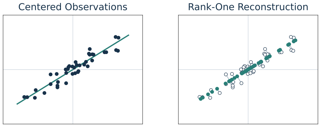
Original-scale reconstruction: \(\widehat{\widetilde{\boldsymbol{x}}}_i=\boldsymbol{\mu}+W\boldsymbol{z}_i\).

Synthetic example, not cell measurements. The second panel shows reconstruction back in two dimensions, not the one-dimensional feature coordinate itself. The short perpendicular segments are exactly the errors the PCA objective measures.

A curved structure can be low-dimensional without being linear

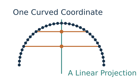
Would one linear feature reconstruct every point exactly? Could a nonlinear coordinate do so? What does “one-dimensional” mean in each claim?

Pairs, 3 minutes. A curved arc can be parameterized by one angle, but no straight line contains it, so one-dimensional linear reconstruction cannot be exact. This particular vertical projection also creates collisions; do not claim every linear projection of a semicircle has collisions. A horizontal coordinate on this upper semicircle is injective, but its exact decoder would be nonlinear.

PCA solves the stated problem; usefulness still needs evidence

• Chosen objective: squared error in the selected measurements and units.
• Mathematical solution: leading right singular vectors of centered data.
• Remaining questions: which features and preprocessing, how many components, and whether the retained variation matters for the intended use.

Next: translate this mathematical contract into arrays and reliable numerical computation—then ask what the observed data justify claiming about new cases.

Return to the cell-expression anchor: a faithful reconstruction is evidence for this proxy, not automatically for cell type, biological mechanism, or future prediction. Stop the math section here; the next topic introduces NumPy, vectorization, numerical stability, and empirical interpretation.