NumPy and Numerical Computation for PCA

David I. Inouye

Dynamic Content · Last Updated: September 17, 2026

Draft for instructor review. Assumes the completed reconstruction/PCA topic: centering, orthonormal projection, SVD, and the discarded-energy formula. The outline lives in redesign/arc-02-formalization-representation.md. This is a conceptual topic, not a commitment to one class meeting.

The PCA equations give us a computation to implement

Let \(\widetilde X\in\mathbb R^{n\times d}\) contain the original observations as rows.

Operation	Mathematics	Shape
Center	\(X=\widetilde X-\boldsymbol{1}\boldsymbol{\mu}^T\)	\(n\times d\)
Choose directions	\(X=U\Sigma V^T\), \(W=V_k\)	\(d\times k\)
Encode	\(Z=XW\)	\(n\times k\)
Reconstruct	\(\widehat{\widetilde X}=ZW^T+\boldsymbol{1}\boldsymbol{\mu}^T\)	\(n\times d\)

Route: represent the objects, implement the operations, check the numerical result.

Use real-valued finite measurements throughout, n>1 and 1<=k<=min(n,d). The vector of ones has n entries. In code, A represents original data and X represents centered data, preserving the preceding topic’s meaning of X. The mean is estimated column by column. NumPy details serve these equations.

Lists and arrays give different meanings to *

import numpy as np

values = [2, 5, 8]
x = np.array(values, dtype=np.float64)

print("type(values):", type(values))
print("type(x):", type(x))
print(f"values * 2: {values * 2!r}")
print(f"x * 2: {x * 2!r}")
print("x.shape:", x.shape)
print("x.dtype:", x.dtype)

type(values): <class 'list'>
type(x): <class 'numpy.ndarray'>
values * 2: [2, 5, 8, 2, 5, 8]
x * 2: array([ 4., 10., 16.])
x.shape: (3,)
x.dtype: float64

• A list is a Python sequence. Multiplication by an integer repeats it.
• An array stores values with a common data type. Here multiplication scales each entry.
• shape describes the axes. dtype describes how entries are stored.

This is the minimum container bridge, not a general Python tutorial. Use float64 explicitly in these examples so precision comparisons are deliberate. [Sources] source:numpy-array-basics-2026 — array creation, shape, and dtype.

A one-dimensional array has no row or column axis to swap

Shapes: (d,) = one observation; (n, d) = observations × features; (b, n, d) adds a batch axis.

x = np.array([2., 5., 8.])
print("x.shape:", x.shape)
print("x.T.shape:", x.T.shape)
print("x[:, None].shape:", x[:, None].shape)
print("x[None, :].shape:", x[None, :].shape)

x.shape: (3,)
x.T.shape: (3,)
x[:, None].shape: (3, 1)
x[None, :].shape: (1, 3)

• None (equivalently np.newaxis) inserts a length-one axis at that position.
• x[:, None] makes a column; x[None, :] makes a row.
• For 2D arrays, .T swaps the row and column axes.

Indexing: A[i, :] selects observation \(i\); A[:, j] selects feature \(j\).

None inserts an axis of length one. Distinguish a mathematical vector’s role from its storage convention. Keep all PCA batches explicitly two-dimensional. [Sources] source:numpy-array-basics-2026 — adding axes and transposing arrays.

* multiplies entries; @ implements matrix multiplication

P = np.array([[1., 2.],
              [3., 4.]])
Q = np.array([[2., 0.],
              [1., 2.]])
print("P * Q (entrywise):\n", P * Q)
print("P @ Q (matrix product):\n", P @ Q)

P * Q (entrywise):
 [[2. 0.]
 [3. 8.]]
P @ Q (matrix product):
 [[ 4.  4.]
 [10.  8.]]

For PCA, Z = X @ W maps (n, d) @ (d, k) to (n, k).

The upper-left entries are \(1\cdot2=2\) and \(1\cdot2+2\cdot1=4\). Both results have shape (2, 2). Shape alone cannot tell us which operation we intended.

Centering averages across observations for each feature

For each feature, \(\mu_j=\frac1n\sum_{i=1}^n\widetilde X_{ij}\).

A = np.array([[2., 10.],
              [4., 14.], [6., 18.]])
mu = A.mean(axis=0)
X = A - mu
print("mu (feature means):", mu)
print("X (centered data):\n", X)

mu (feature means): [ 4. 14.]
X (centered data):
 [[-2. -4.]
 [ 0.  0.]
 [ 2.  4.]]

Axis rule: count positions in the shape tuple from zero. Aggregate over the chosen dimension and remove it by default. The resulting shapes are:

T = np.zeros((2, 3, 4))
print("T.shape:", T.shape)
print("axis=0:", T.mean(axis=0).shape)
print("axis=1:", T.mean(axis=1).shape)
print("axis=2:", T.mean(axis=2).shape)

T.shape: (2, 3, 4)
axis=0: (3, 4)
axis=1: (2, 4)
axis=2: (2, 3)

Why does X = A - mu work? Ordinary matrix subtraction requires equal shapes. A matrix minus a vector is undefined. NumPy supplies broadcasting.

Trace the first column numerically before considering the whole matrix. Do not imply these synthetic values are actual cell measurements. For A, axis=0 aggregates observations and leaves features; axis=1 would aggregate features within each observation. For T, point to positions 0, 1, and 2 of (2,3,4): removing them gives (3,4), (2,4), and (2,3). Zeros keep attention on shapes rather than values. These output shapes use the default keepdims=False; the broadcasting section introduces keepdims=True. [Sources] source:numpy-array-basics-2026 — reductions over axes.

Broadcasting compares dimensions from right to left

At each position, either of two rules must hold:

1. The two dimension sizes are equal: keep that size.
2. One size is 1: reuse its value along the other dimension’s size.

Missing dimensions count as 1s (marked * below). If neither rule holds at any position, broadcasting fails.

Vector (4,)

(3, 4)
(*, 4)
------
(3, 4)

Matrix (3, 1)

(2, 3, 4)
(*, 3, 1)
---------
(2, 3, 4)

Both inputs expand

(3, 1)
(1, 4)
------
(3, 4)

Scalar ()

(2, 3, 4)
(*, *, *)
---------
(2, 3, 4)

Vector (3,): incompatible

(3, 4)
(*, 3)
------
 Error

Rightmost sizes 4 and 3 are neither equal nor 1.

Point to the rightmost pair first in every row. Missing dimensions mean missing leading positions after right alignment, not arbitrary gaps between axes. For (2,3,4) and (3,1): compare 4 with 1, then 3 with 3, then 2 with a missing 1. Dimension sizes in these teaching examples are positive. The star is a diagram placeholder, not literal NumPy shape syntax. Raw input shapes are shown above each stack; placeholders make absent leading axes visible. [Sources] source:numpy-broadcasting-2026 — general broadcasting rules.

Mathematics makes the repeated mean an explicit matrix

\[ \underbrace{X}_{n\times d} =\underbrace{\widetilde X}_{n\times d} -\underbrace{\boldsymbol{1}_n\boldsymbol{\mu}^T}_{(n\times1)(1\times d)=n\times d}. \]

In NumPy, A - mu produces the same entries: \(X_{ij}=\widetilde X_{ij}-\mu_j\).

ones = np.ones((A.shape[0], 1))
mu_matrix = ones @ mu[None, :]
print("mu_matrix:\n", mu_matrix)
print("A - mu:\n", A - mu)
print("Same result:",
      np.allclose(A - mu_matrix, A - mu))

mu_matrix:
 [[ 4. 14.]
 [ 4. 14.]
 [ 4. 14.]]
A - mu:
 [[-2. -4.]
 [ 0.  0.]
 [ 2.  4.]]
Same result: True

A: (3, 2); mu: (2,). Broadcasting avoids copying the repeated means, saving allocation and memory traffic. The output still needs storage.

The vector of ones makes the subtraction well-defined in ordinary matrix algebra. Its product with the row vector of feature means repeats that row n times. We construct it here only to connect the equation with the broadcast computation. np.allclose checks the agreement on this example; the entrywise identity explains why they agree generally. The output X still needs n-by-d storage. [Sources] source:numpy-broadcasting-2026 — conceptual expansion without copying operands.

keepdims=True preserves reduced axes with length one

For T.shape == (2, 3, 4), reducing axis=1 gives (2, 4) by default. With keepdims=True, it gives (2, 1, 4): the reduced position stays explicit.

reduced = T.mean(axis=1)
kept = T.mean(axis=1, keepdims=True)
restored = reduced[:, None, :]
print("T.shape:", T.shape)
print("reduced.shape:", reduced.shape)
print("kept.shape:", kept.shape)
print("restored.shape:", restored.shape)
print("(T - kept).shape:", (T - kept).shape)

T.shape: (2, 3, 4)
reduced.shape: (2, 4)
kept.shape: (2, 1, 4)
restored.shape: (2, 1, 4)
(T - kept).shape: (2, 3, 4)

• keepdims preserves a reduced axis; None inserts a new axis where specified.
• (2, 1, 4) broadcasts back against (2, 3, 4).
• (2, 4) would align as (1, 2, 4) and fail at the middle position.

The mean values are the same in reduced, kept, and restored; their shapes differ. Use the zero-valued tensor from the earlier axis example so only the shapes are at issue. Indexing with None or np.newaxis inserts a view axis rather than repeating values. The missing middle singleton cannot be inferred by the right-to-left rule; only missing leading positions receive implicit ones. [Sources] source:numpy-array-basics-2026 — adding axes and keeping reduced dimensions. source:numpy-broadcasting-2026 — alignment from the right.

Division broadcasts one standard deviation per feature

For positive feature standard deviations \(s_j\), \(H_{ij}=(\widetilde X_{ij}-\mu_j)/s_j\). In matrix notation, \(H=X\operatorname{diag}(1/s_1,\ldots,1/s_d)\).

std = A.std(axis=0)
H = (A - mu) / std
H_mul = (A - mu) * (1 / std)
print("std:", std.round(3))
print("H.round(3):\n", H.round(3))
print("H.std(axis=0):", H.std(axis=0))
print("Division equals multiplication:",
      np.allclose(H, H_mul))

std: [1.633 3.266]
H.round(3):
 [[-1.225 -1.225]
 [ 0.     0.   ]
 [ 1.225  1.225]]
H.std(axis=0): [1. 1.]
Division equals multiplication: True

(3, 2) / (2,) reuses each feature’s scale across observations. The same shape rules apply to elementwise +, -, *, and /. Scaling changes the relative weight of features in PCA’s reconstruction error.

This example uses NumPy’s default ddof=0, dividing variance by n. Both columns have positive standard deviation. A constant feature needs separate treatment before division. The arithmetic illustrates broadcasting, not a recommendation that all gene-expression features should be standardized. Scaling changes the PCA objective by weighting squared errors inversely by feature scale squared. Matrix @ has its own contracted-dimension rules; do not apply elementwise rules to those axes. [Sources] source:numpy-broadcasting-2026 — elementwise arithmetic with broadcast operands.

Code can run successfully while centering the wrong objects

A = np.array([[2., 10.],
              [4., 14.], [6., 18.]])
B = A - A.mean(axis=1, keepdims=True)
print("B:\n", B)
print("B.mean(axis=1):", B.mean(axis=1))
print("B.mean(axis=0):", B.mean(axis=0))

B:
 [[-4.  4.]
 [-5.  5.]
 [-6.  6.]]
B.mean(axis=1): [0. 0. 0.]
B.mean(axis=0): [-5.  5.]

What does this code subtract? Which averages become zero? Would this prepare the data for the PCA problem we defined? Repair the expression and explain why.

Pairs, 3 minutes plus a short debrief. Diagnose meaning rather than syntax. The code subtracts each observation’s average across its two features. Every row mean is zero, while the feature means need not be zero. Repair with axis=0, with or without keepdims. Distinct n and d prevent an accidental square-matrix match from distracting from the conceptual error.

NumPy returns the right singular vectors as rows of Vt

U, s, Vt = np.linalg.svd(
    X, full_matrices=False)
W = Vt[:k, :].T

full_matrices=False omits extra directions multiplied by zero rows or columns of rectangular \(\Sigma\). This reduced SVD keeps \(m=\min(n,d)\) singular values; selecting the first \(k\) is a separate truncation.

Returned array	Shape	Mathematical role
U	(n, m)	Left singular vectors
s	(m,)	Singular values, largest first
Vt	(m, d)	Rows are right singular vectors transposed
W	(d, k)	First \(k\) right singular vectors as columns

The argument False requests reduced shapes, not a rank-k approximate solver. The routine still computes all min(n,d) singular values. Rank may be smaller than m. We restrict k to 1..m. For complex input the output is the conjugate transpose, but this lecture uses real data. The variable name Vt is our choice. [Sources] source:numpy-svd-2026 — return values and full_matrices.

Encoding and reconstruction follow the same equations as before

Xraw stores \(\widetilde X\), the original observations.

Xraw = np.array([[2., 10.], [4., 15.],
                 [6., 17.], [8., 22.]])
mu = Xraw.mean(axis=0)
X = Xraw - mu
U, s, Vt = np.linalg.svd(
    X, full_matrices=False)
k = 1
W = Vt[:k, :].T
Z = X @ W
Xraw_hat = Z @ W.T + mu
print("Z.round(3):\n", Z.round(3))

Z.round(3):
 [[-6.708]
 [-1.347]
 [ 1.347]
 [ 6.708]]

For \(X\in\mathbb R^{n\times d}\) and \(W\in\mathbb R^{d\times k}\), \(\widehat X=(XW)W^T=X(WW^T)\).

Centered reconstruction	Arithmetic cost	Intermediate
Xhat = (X @ W) @ W.T	\(O(ndk)\)	\(n\times k\)
Xhat = X @ (W @ W.T)	\(O(d^2k+nd^2)\)	\(d\times d\)

This is the complete small dense PCA computation, with finite real input and valid k assumed. Ask students to identify the encoder and decoder. Vectorization: X @ W computes all observations together. With standard dense multiplication, the first grouping costs ndk + nkd = 2ndk operations up to constant factors. The second costs dkd + ndd. For k much smaller than d, using the coordinates avoids the large d-by-d projection matrix. Costs exclude the preceding SVD and restoring the mean; Xhat here is centered. Subtracting the original-scale arrays measures the same residual as X-Z@W.T. [Sources] source:numpy-svd-2026 — reduced SVD reconstruction.

The computed arrays show PCA’s shapes and reconstruction

print("X.shape:", X.shape)
print("U.shape:", U.shape)
print("s.shape:", s.shape)
print("Vt.shape:", Vt.shape)
print("W.shape:", W.shape)
print("Z.shape:", Z.shape)
print("Xraw_hat.shape:", Xraw_hat.shape)
print("s.round(4):", s.round(4))
print("Xraw_hat.round(3):\n",
      Xraw_hat.round(3))
error = np.sum((Xraw - Xraw_hat)**2)
print(f"error (squared): {error:.6f}")

X.shape: (4, 2)
U.shape: (4, 2)
s.shape: (2,)
Vt.shape: (2, 2)
W.shape: (2, 1)
Z.shape: (4, 1)
Xraw_hat.shape: (4, 2)
s.round(4): [9.6755 0.6201]
Xraw_hat.round(3):
 [[ 1.923 10.04 ]
 [ 4.382 14.803]
 [ 5.618 17.197]
 [ 8.077 21.96 ]]
error (squared): 0.384552

We retained one direction, but full_matrices=False still computed both singular values.

Continue the preceding four-observation, two-feature example. Reduced factor shapes are distinct from a solver that computes only k components. [Sources] source:numpy-svd-2026 — reduced SVD shapes.

New observations use the fitted mean and directions

# Apply the representation fitted on Xraw
Xraw_new = np.array([[5., 16.], [7., 20.]])
Z_new = (Xraw_new - mu) @ W
Xraw_new_hat = Z_new @ W.T + mu
print("Z_new.round(3):\n", Z_new.round(3))
print("Xraw_new_hat.round(3):\n",
      Xraw_new_hat.round(3))

Z_new.round(3):
 [[0.   ]
 [4.472]]
Xraw_new_hat.round(3):
 [[ 5.    16.   ]
 [ 7.051 19.974]]

• Fitting estimates mu and W from a chosen dataset.
• Applying uses those fixed values for other observations with the same feature definitions.
• Re-estimating the mean or directions creates a different fitted representation.

PCA relies on centering and then measuring variance. What would happen if we computed variance directly, without centering first?

Students have not yet studied train/validation/test methodology. Establish the fit/apply distinction now, then let Arc 3 justify independent evaluation. If optional feature scaling is used, save and reuse the fitted scales as well.

Computing spread for PCA starts with an exact identity

For one feature’s values \(x_1,\ldots,x_n\), let \(\bar x=\frac1n\sum_{i=1}^{n}x_i\). The mean \(\bar x\) is constant with respect to \(i\).

\(\displaystyle \frac1n\sum_{i=1}^{n}(x_i-\bar x)^2\)

\(=\)

\(\displaystyle \frac1n\sum_{i=1}^{n}\bigl(x_i^2-2x_i\bar x+\bar x^2\bigr)\)

(Expand the square inside the sum)

\(\,\)

\(=\)

\(\displaystyle \frac1n\sum_{i=1}^{n}x_i^2-\frac{2\bar x}{n}\sum_{i=1}^{n}x_i+\frac1n\sum_{i=1}^{n}\bar x^2\)

(Distribute the sum; pull out constants)

\(\,\)

\(=\)

\(\displaystyle \frac1n\sum_{i=1}^{n}x_i^2-\frac{2\bar x}{n}(n\bar x)+\frac1n(n\bar x^2)\)

(\(\sum_{i=1}^{n}x_i=n\bar x\); \(n\) copies of \(\bar x^2\))

\(\,\)

\(=\)

\(\displaystyle \frac1n\sum_{i=1}^{n}x_i^2-2\bar x^2+\bar x^2\)

(Cancel the factors of \(n\))

\(\,\)

\(=\)

\(\displaystyle \frac1n\sum_{i=1}^{n}x_i^2-\bar x^2\)

(Combine terms)

Motivate from PCA: our mathematical variance interpretation and centering step now have to be evaluated on a finite-precision computer. Is algebraic correctness enough? Reduce to one feature and five numbers; this is the only worked failure. This is the average squared deviation of a finite list, using divisor n, not an expectation over a probability distribution or the n-1 sample estimator. Every sum runs from 1 through n. Explicitly point out that the constant term occurs n times. Reveal one algebraic operation at a time before asking whether its numerical implementations will agree.

Will mathematically equivalent computations give the same answer?

Take the five numbers \(10^9+1,\ldots,10^9+5\). Their mean is \(10^9+3\). What variances will the two computations report? Predict before revealing.

v = 1e9 + np.arange(1., 6.)
centered = v - v.mean()
center_first = np.mean(centered**2)
subtract_totals = np.mean(v**2) - v.mean()**2
print("Centered:", center_first)
print("Raw squares:", subtract_totals)

Centered: 2.0
Raw squares: 0.0

Choice	Centered	Raw squares
A	\(2\)	\(2\) (up to a tiny rounding error)
B	\(2\)	\(0\)
C	\(2\)	Overflow: the squared values are too large

Individual prediction, then a short pair discussion (about two minutes). Vote A, B, or C, then reveal the labeled outputs. B is correct. A expresses the expectation that any numerical difference must be tiny; C confuses loss of precision with exceeding the representable range. These squared values are within float64’s range: this example loses a small difference, not range. Both formulas are exactly equal in real arithmetic. On this float64 example the first gives 2.0 and the second 0.0. The original numbers are exactly representable; the failure occurs in computing the large squared quantities. Do not introduce another example or a different PCA solver.

Numerical errors can erase the entire answer

print("Centered values:", centered)
print("Mean of squares:", np.mean(v**2))
print("Square of mean:", v.mean()**2)
print("Centered:", center_first)
print("Raw squares:", subtract_totals)

Centered values: [-2. -1.  0.  1.  2.]
Mean of squares: 1.000000006e+18
Square of mean: 1.000000006e+18
Centered: 2.0
Raw squares: 0.0

• Centering first gives \((-2,-1,0,1,2)\): the mean square is \((4+1+0+1+4)/5=2\).
• The other formula subtracts rounded values near \(10^{18}\). The small difference is lost: catastrophic cancellation.
• This is 100% relative error: zero instead of two, not just a changed last decimal.

Numerical stability: choose computations that control the effect of rounding errors. A correct mathematical formula alone does not ensure a reliable computation.

Later: log probabilities help avoid tiny probabilities rounding to zero; softmax needs careful implementation to avoid overflow.

The two large computed terms round to the same float64 number in this example. Subtraction exposes the lost information; it cannot recover it. Centering first avoids the large intermediate squares here. It does not recover information already rounded away in input data. Keep the discussion at the principle level: mathematical equivalence does not guarantee numerical equivalence. This is the first explicit math-versus-computation lesson: numbers have finite precision, intermediate results are rounded, and the final error can be large. Connect back to PCA: the computation of means, variance, and reconstruction is part of the algorithm, not merely transcription of an equation. Stable methods limit amplification of rounding; no claim that all PCA implementations fail. The future hints are not worked examples. Later use sums of log probabilities rather than products of tiny probabilities, and a shifted softmax that avoids large positive exponentials. Do not derive either here.

From computing PCA to interpreting real data

Back to our original question: what should a useful representation preserve?

We can now compute PCA. Does it reveal useful structure in real gene-expression data?

Pause to close the numerical-computation section and return to the original representation problem. Next compare PCA with random projections, inspect how much variance is retained, and ask what the annotations let us conclude.

PCA reveals known cell-line structure without seeing the labels

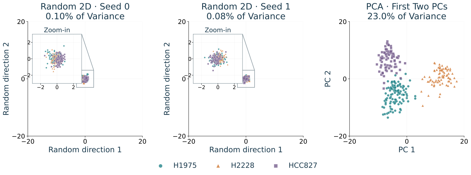
Real gene expression: 274 cells from three lung-cancer cell lines; 2,000 selected genes per cell.

[Sources] - source:scmixology-readme-2019 — experiment description and annotation definitions. - source:scmixology-celseq2-counts-2019 — complete post-author-QC CEL-seq2 matrix. - source:scmixology-celseq2-metadata-2019 — cell_line_demuxlet annotations. - source:scmixology-license-2019 — MIT license in the author repository.

These are cultured human lung adenocarcinoma cell lines, not patient groups or newly discovered cell types. Gene expression measures RNA abundance, not DNA genotype. Use all 274 source-QC cells: H1975 112, H2228 81, HCC827 81. Remove non-ENSG controls, retain genes detected in at least three cells, normalize each cell’s gene counts to total 10,000 and apply log(1+x). Select the 2,000 highest-variance transformed genes, then center each gene. Do not scale each gene to unit variance. Selection, centering, SVD and random directions never use cell-line labels. This is our simple teaching analysis, not a reproduction of the paper’s pipeline. Random directions are QR-orthonormalized Gaussian columns, seeds 0 and 1 fixed before inspection. They are a random-subspace baseline with the same encoder/ decoder geometry as PCA, not a distance-rescaled Gaussian embedding. The variance fraction is squared projected norm divided by total centered squared norm. All three main panels share identical x/y limits and equal unit scales. The two random projections also have matched zoom-in insets (both axes -3 to 3), showing that their small spread is not hiding clear cell-line separation. Do not claim every random projection fails or that PCA always separates labels. Reproduce with lectures/scripts/scmixology_case.py. Data and analysis-code hashes key the local cache; lecture rendering only reads local vector figures.

Log-normalized expression; labels only color the points. Shared main axes; matching zoom-in scales. Data: Tian et al., scMixology (2019), CEL-seq2.

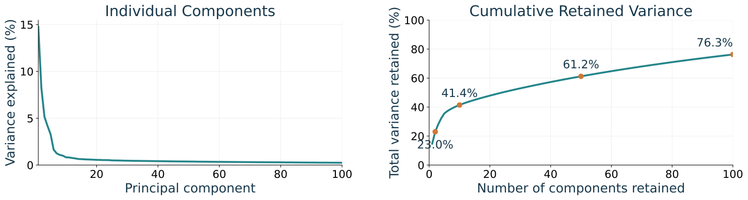
Two PCs reveal groups but retain only 23% of the variance

\[\text{Retained fraction}(k)=\frac{\sum_{j=1}^{k}\sigma_j^2}{\sum_{j=1}^{r}\sigma_j^2},\qquad r=\operatorname{rank}(X).\]

• Visualization: two coordinates already reveal cell-line structure.
• Reconstruction: 100 PCs retain 76.3%; reaching 90% requires 173 PCs.

[Sources] - source:scmixology-celseq2-counts-2019

All percentages refer to the same 274-by-2,000 centered, log-normalized matrix, not raw counts, all measured genes, or biological information. The denominator uses the full SVD spectrum, not just the first 100 components shown. Reducing 2,000 features to 100 retains 76.2775% of centered energy. The 90% threshold is an illustration, not a recommended universal rule. Components beyond 100 are computed but not plotted; the threshold occurs at 173. No new derivation. The small last singular value reflects centering; numerical residual energy is negligible. Ask how visualization and reconstruction lead to different k choices.

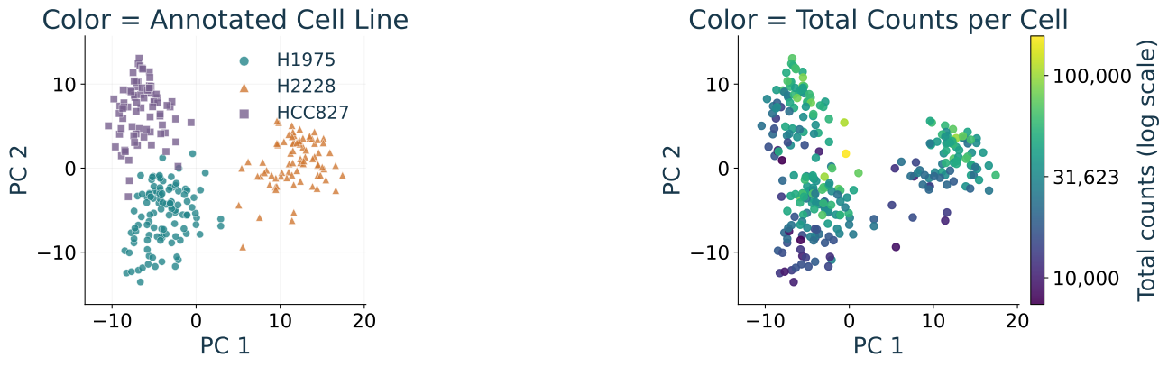
The same PCA plot supports different questions about usefulness

Discuss: Do these plots justify saying that PCA preserved the biology we care about?

• What does agreement with known cell-line labels support?
• What might total counts per cell explain—and what evidence would you want next?

[Sources] - source:scmixology-readme-2019 - source:scmixology-celseq2-counts-2019 - source:scmixology-celseq2-metadata-2019

Merged interpretation and evidence activity, about two minutes. These are the same coordinates, recolored after fitting. Left: labels supply an external annotation consistent with the visible groups; they did not train PCA. Right: total endogenous-gene counts before normalization vary across cells and still track some position within groups. Such counts can reflect both capture depth and biological RNA content. Color association alone does not establish a technical artifact or a biological cause, nor prove normalization has failed. We used one protocol, so this is not a claim about between-protocol batch effects. Seek known markers, independent measurements, replicate experiments, and a specified downstream purpose. Do not assume held-out evaluation terminology yet. The plot supports structure in this sample; it does not establish all relevant biology, disease prediction, a causal explanation, or future performance.

We fitted these observations; new cells need new evidence

From the original question…	…to what we established
Make thousands of measurements easier to inspect	Choose what the representation should preserve
Preserve observations under a squared-error criterion	PCA gives the best rank-\(k\) linear reconstruction
Compute that representation	Center, use SVD, and attend to finite precision
Inspect this cell dataset	Two PCs reveal known groups, but retain only 23% of variance

For new cells: keep the fitted preprocessing, gene set, mean, and directions fixed.

Before moving on: what general lessons does this case teach us about building useful representations?

[Sources] - source:scmixology-celseq2-counts-2019

The case wraps the arc: purpose, formalization, solution, numerical computation, and interpretation. New cells must use the same measurement definitions and preprocessing rule; reuse selected genes, fitted means, and PCA directions. This analysis used every cell for fitting and makes no held-out performance claim. The closing question opens the broader task of turning representations into useful predictions, discoveries, or decisions and evaluating those uses. Generalization is one part of that larger question, not the only destination. Do not start a train/test or classifier tutorial here. The following retrospective connects this case to the principles developed across the arc.

A useful solution begins with deciding what to preserve

Gene-expression measurements → desired representation → objective → constraints → solution

Choice we made	What it allowed us to specify
Which measurements, preprocessing, and units?	The observations and geometry
What should the representation preserve?	Squared reconstruction error
Which transformations are allowed?	A linear representation with \(k\) coordinates
What is the best solution under those choices?	Leading right singular vectors of centered data

Formalization makes a vague goal solvable. Choosing the goal remains our responsibility.

Arc-level synthesis, not a new derivation. Revisit the full chain from the original cell-data question. PCA’s optimality is conditional on the objective, representation, and constraints; it does not choose those for us.

Representations preserve some structure and discard other structure

In our cell-expression example	What it teaches us
Two PCs reveal known cell-line groups	A small representation can expose useful structure
Those two PCs retain only 23% of variance	Visible groups do not imply faithful reconstruction
100 PCs retain 76.3% of variance	The number of coordinates depends on the purpose

• Rank and discarded singular values describe linear information loss.
• Low-dimensional structure need not be linear: recall the curved-data example.
• Large variance is not automatically the variation that matters for our task.

Ask what was preserved, what was lost, and whether that matches the intended use.

[Sources] - source:scmixology-celseq2-counts-2019

Percentages refer to the same centered 274-by-2,000 log-normalized matrix used in the case. This summarizes the figures students just inspected. Distinguish linear reconstruction dimension from a useful two-coordinate visualization.

A proof, a working computation, and useful evidence are different achievements

Question	What this arc established
Did we solve the stated problem?	SVD gives the optimal linear PCA reconstruction
Did we compute it correctly and efficiently?	Shapes, broadcasting, operation order, and finite precision matter
Does the result accomplish our purpose?	Real-data evidence supports particular claims, with limits

A mathematical guarantee does not establish every practical claim we might want to make.

Next question: What evidence would justify trusting a learned rule on new observations?

Close Arc 2 before opening a predictor example in Arc 3. A correct numerical implementation can produce a representation that is not useful for a chosen purpose. A useful plot of fitted observations does not by itself establish performance for future observations. Do not teach train/validation/test here.