Binary Prediction: Goals and Historical Data

David I. Inouye

Last updated: September 22, 2026

What would justify trusting a prediction for someone we have never seen?

Opening of Arc 3. This topic formalizes the goal before introducing historical training data or methods. The complete arc outline is tentative. This opening stops at the question that motivates KNN; do not teach evaluation procedures yet.

Different settings ask the same kind of prediction question

Setting	Prediction question with two possible answers
Bank phone campaign	Will this customer open a term-deposit account?
Wine screening	Will this wine receive a high sensory rating?
Activity recognition	Is this person walking?

Each uses information available now to predict an outcome we do not yet know.

Our running case: the bank phone campaign. A term-deposit account holds money for a fixed period to earn interest.

[Sources] - source:uci-bank-marketing - source:uci-wine-quality - source:uci-smartphone-activity

These are three real dataset settings. The bank case uses UCI Bank Marketing, whose label describes taking up a term deposit, not a credit-card application. Explain the product before using the shorter phrase “open the account.” For the proposed wine binary task, define high rating as a sensory score >=7; this cutoff is our choice, not a universal commercial standard. For the sensor example, recode WALKING, WALKING_UPSTAIRS, and WALKING_DOWNSTAIRS as walking, and SITTING, STANDING, LAYING as not walking. State the recoding if asked. Original wine labels are ordinal and original HAR labels have six classes. At this stage the sensor question concerns an unknown current activity, not necessarily forecasting a future event. Inputs need not be images.

Each practical question needs a mathematical counterpart

Practical question	Bank-case answer	Mathematical counterpart
What information is available?	New customer information known before the call	?
What answer do we want?	Whether the customer opens the offered account	?
What makes a predictor good?	Few mistakes across unseen customers	?

We will fill in one mathematical counterpart at a time.

[Sources] - source:uci-bank-marketing

The source calls the outcome “subscribed a term deposit.” Use “opened the offered term-deposit account” as the plain-language explanation. This is the recorded campaign outcome, not necessarily the result of one call; campaigns may include multiple contacts. Do not invent a 30-day window. This predicts response, not the causal effect of calling. Equal mistake costs are the initial modeling choice. Read the first two columns from left to right. The question marks create three specific gaps that the following slides fill in this same row order.

Available information becomes the input \(\boldsymbol{x}\)

Question: What information is available?

Bank-case answer: New customer information known before the call.

Formalization:

\[\boldsymbol{x}\in\mathcal X\]

\(\boldsymbol{x}\) is one customer’s available information; \(\mathcal X\) is the set of valid input representations.

This fills the first row of the opening map. Examples include age, job, and information from completed prior campaigns if known before the call. Not every attribute must already be numerical. We will decide how to encode information when a method requires it. Do not introduce the training dataset yet.

The desired answer becomes the output \(y\)

Question: What answer do we want?

Bank-case answer: Whether the customer opens the offered account.

Formalization:

\[ \boldsymbol{x} \quad\xrightarrow{\quad f\quad}\quad \widehat y\in\{0,1\} \]

\(y\in\{0,1\}\) is the actual outcome. The prediction is correct when \(\widehat y=y\).

This fills the second row of the opening map. The predictor f receives the available input and returns a predicted outcome. Keep prediction \(\widehat y\) distinct from actual outcome y. The actual outcome may be observed later, but the framework also covers outcomes that are already determined and merely unseen. No training process or algorithm has been defined.

Population error formalizes few mistakes on unseen customers

A distribution \(p\) describes how common different unseen customer–outcome pairs are. A random pair \((\mathbf{x},\textnormal{y})\) drawn from \(p\) contains the available information and what actually happens.

The population error is the chance that our prediction is wrong:

\[ R_p(f)=\Pr_{(\mathbf{x},\textnormal{y})\sim p} \bigl(f(\mathbf{x})\ne\textnormal{y}\bigr). \]

Goal: choose \(f^*\in\operatorname*{arg\,min}_{f:\mathcal X\to\{0,1\}} R_p(f)\).

This completes the goal—but it does not tell us how to find \(f\).

p is the unknown joint distribution of inputs and outcomes, not a dataset or a known table. Explain probability in words before reading the equation. Argmin means a predictor attaining the smallest error; we are not deriving the Bayes classifier here. Do not assume the minimum is zero or that every outcome is fully determined by the available input. No empirical average or train/test split is introduced yet. The goal can be defined without assuming i.i.d. historical data; that assumption enters when using historical data to address it.

The prediction contract now has a mathematical form

Practical question	Bank-case answer	Mathematical counterpart
What information is available?	New customer information known before the call	Input \(\boldsymbol{x}\in\mathcal X\)
What answer do we want?	Whether the customer opens the offered account	Outcome \(y\in\{0,1\}\); prediction \(\widehat y=f(\boldsymbol{x})\)
What makes a predictor good?	Few mistakes across unseen customers	Small population error \(R_p(f)\)

The unresolved question: How do we find the right function \(f\)?

Return to exactly the same map shown with question marks. Read the completed third column top to bottom and emphasize the unresolved question. This is the concise synthesis of the prediction contract, not a new inventory.

Machine learning infers the rule \(f\) from examples

In ordinary computation, the rule is given. For example, a circuit simulator is given equations and parameters, then computes an output from an input.

Ordinary computation

\[f\ \text{given},\qquad \boldsymbol{x}\longmapsto f(\boldsymbol{x})\]

Machine learning

\[\mathcal D=\{(\boldsymbol{x}_i,y_i)\}_{i=1}^{n} \quad\longmapsto\quad \text{infer } f\]

The historical input–outcome pairs \(\mathcal D\) are the training data. They give examples of the mapping, but not the rule itself.

[Sources] - source:uci-bank-marketing

This is the central conceptual hinge. Many conventional programs are supplied with a rule or procedure: a simulator is given governing equations and a sorting routine is given its ordering procedure. Machine learning instead receives example inputs paired with observed outputs and must construct a rule that also works for unseen inputs. Do not imply that the inferred rule is unique or that training examples alone guarantee success.

A dataset column is not automatically an allowed input

Prediction moment: before calling this customer.

Historical columns: recorded age and job · duration of last call · whether the customer opens this account

Can call duration be used to predict whether this customer will open the account before the call begins?

A. Yes, because it appears in the historical training data.

B. Yes, if the historical dataset is sufficiently large.

C. No, because it is unavailable at the prediction moment.

Larger principle: available columns describe a dataset; allowed inputs are determined by the real decision we are trying to support.

[Sources] - source:uci-bank-marketing - source:uci-bank-marketing-data

This subtle distinction deserves emphasis but not a long detour. Pairs, about two minutes. Although the dataset calls this the last contact duration, the value for each row is recorded only after the contact whose outcome appears in that row. Use that temporal detail during the discussion rather than revealing it in the table. More records do not repair the mismatch. Other fields need the same prediction-time audit. This is a problem-formulation issue, not merely a later data-cleaning step.

Assumptions mark where a learned predictor can break

Training pairs are the evidence. Performance on unseen pairs is the claim. An explicit assumption must connect them:

\[ \underbrace{\text{training pairs}}_{\text{observed evidence}} \quad\xrightarrow{\quad\text{assumption}\quad}\quad \underbrace{\text{unseen pairs}}_{\text{desired claim}} \]

The most common simple starting point is i.i.d. sampling: model the training pairs and unseen pairs as independent draws from the same distribution \(p\).

I.i.d. is deliberately naive. When it reasonably approximates the problem, it provides a useful foundation for analysis. We will use it for now.

Begin from the evidence-to-claim gap before unpacking the letters in i.i.d. Training data alone cannot establish how unseen cases behave. We must state the assumption that licenses the connection. I.i.d. is common because it is simple enough to analyze and often a useful first approximation, not because every real dataset satisfies it. The next two slides make its two parts explicit. Later sections revisit what changes when either part is implausible, including changes to the data unit, evaluation design, or target population.

Independence rules out linked training examples

The first “I” in i.i.d. is independent.

Knowing one sampled pair \((\mathbf{x}_i,\textnormal{y}_i)\) should not change the probability of another draw once the population distribution is fixed. The unseen case should also be independent of the sample used to construct \(f\).

Possible violation: if the same customer appears after several campaign contacts, those rows and outcomes may be linked rather than independent examples.

Start with independence because it is the first I. This is a modeling assumption, not an established fact about the bank dataset. The source states that campaigns may involve multiple contacts, but records are not guaranteed to be unique people; present the repeated-customer example as a possible violation, not a claim about the released rows. Clustered households or coordinated campaigns are other examples, but omit them unless discussion needs one.

Identically distributed connects training pairs to unseen cases

The second “I” in i.i.d. is identically distributed.

Training pairs and the unseen pairs we care about are modeled as draws from the same joint distribution \(p\)—both the inputs and how they relate to the outcome.

Possible violation: if the bank changes who it contacts or changes the offered account, deployment cases may no longer follow the training distribution.

Same distribution does not mean the same customers or repeated feature values.

State the working assumption in plain language: unseen customers resemble past customers in both their available information and how that information relates to opening the offered account. This is stronger than saying the input columns have the same names. A random split cannot establish that unseen deployment cases follow the same distribution.

The contract and evidence now motivate a first method

The contract asks for low error on unseen customers using only information available before the call. Training pairs become evidence under our working assumption that they and the unseen cases are connected.

First idea: find past customers similar to the new customer and consult their outcomes.

Next question: What should “similar” mean, and why should their outcomes help?

This is the transition into KNN, not yet its implementation or evaluation. The next draft will construct a first neighbor-based rule, explain local smoothness, and then ask how to measure its success. Do not imply that merely returning an answer achieves the population optimum or that the historical dataset supplies unseen outcomes directly.

2. How can examples produce a predictor?

KNN makes learning from local evidence visible without making the algorithm the point.

KNN predicts from nearby observed outcomes

For a new customer \(\boldsymbol{x}\):

1. compute the distance to every training input \(\boldsymbol{x}_i\);
2. keep the indices \(\mathcal N_k(\boldsymbol{x})\) of the \(k\) nearest;
3. average their observed outcomes and take a majority vote.

\[ \widehat\eta_k(\boldsymbol{x}) =\frac{1}{k}\sum_{i\in\mathcal N_k(\boldsymbol{x})}y_i, \qquad \widehat y=\mathbb 1\!\left[\widehat\eta_k(\boldsymbol{x})\geq\tfrac12\right]. \]

The method constructs a prediction directly from the stored examples.

Use a small odd value of k for the first verbal example. The average is a local positive fraction; the threshold turns that estimated probability into a binary prediction. Do not optimize k yet. The point is that a learning rule can be constructed from examples without fitting a parametric formula.

Changing the axes can change who is nearest

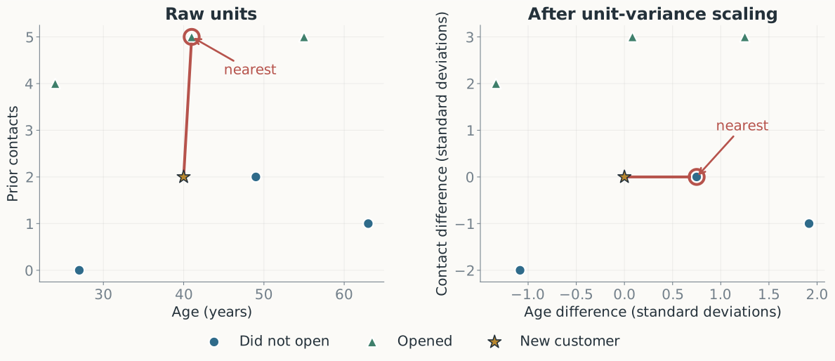
Distance measures differences in the coordinates we supply—not an intrinsic notion of customer similarity.

This is an illustrative bank-campaign example, not a claim about a particular row of the UCI data. The new customer is age 40 with two completed prior contacts. One historical customer differs by one year and three contacts; another differs by nine years and no contacts. Raw Euclidean distance privileges the age unit. After scaling age by 12 years and prior contacts by one contact, the neighbor flips. The plot is generated by lectures/scripts/arc3_knn_figures.py.

Unit-variance scaling is a simple default metric

For each feature \(j\), estimate its training mean and standard deviation, then use

\[ x'_{ij}=\frac{x_{ij}-\widehat\mu_j}{\widehat s_j}. \]

• Apply the same rule to numeric columns and binary indicator columns.
• Encode categorical attributes first—for example, with one indicator per category.
• Estimate \(\widehat\mu_j\) and \(\widehat s_j\) from training data only; remove constant columns.

Interpretation: every retained coordinate has empirical variance one before distance is computed.

This is the most natural baseline when no domain knowledge supplies feature weights. It does not prove that the resulting metric is meaningful. Never assign unordered categories arbitrary integers and then interpret numerical distance. For a binary indicator with prevalence p, the standard deviation is sqrt(p(1-p)); consequently a rare indicator receives a relatively large scaled difference. Mention this only as a reason to validate the metric, not as a new detour. Fit all preprocessing within the training split.

The neighbor fraction estimates a local outcome probability

The population quantity is

\[ \eta(\boldsymbol{x}) =\Pr(\textnormal{y}=1\mid\mathbf{x}=\boldsymbol{x}). \]

KNN substitutes nearby observed outcomes for repeated outcomes at exactly the same input:

\[ \widehat\eta_k(\boldsymbol{x}) =\frac{\text{nearby customers who opened the account}}{k}. \]

Similar customers need not have identical outcomes; their probabilities must be locally related.

The local fraction estimates eta, while the majority vote is the corresponding classification decision under equal mistake costs. Different labels among nearby customers can reflect information not represented in x rather than an algorithmic error. This creates the need for a local-smoothness argument.

With more data, \(k\) can grow while neighborhoods stay local

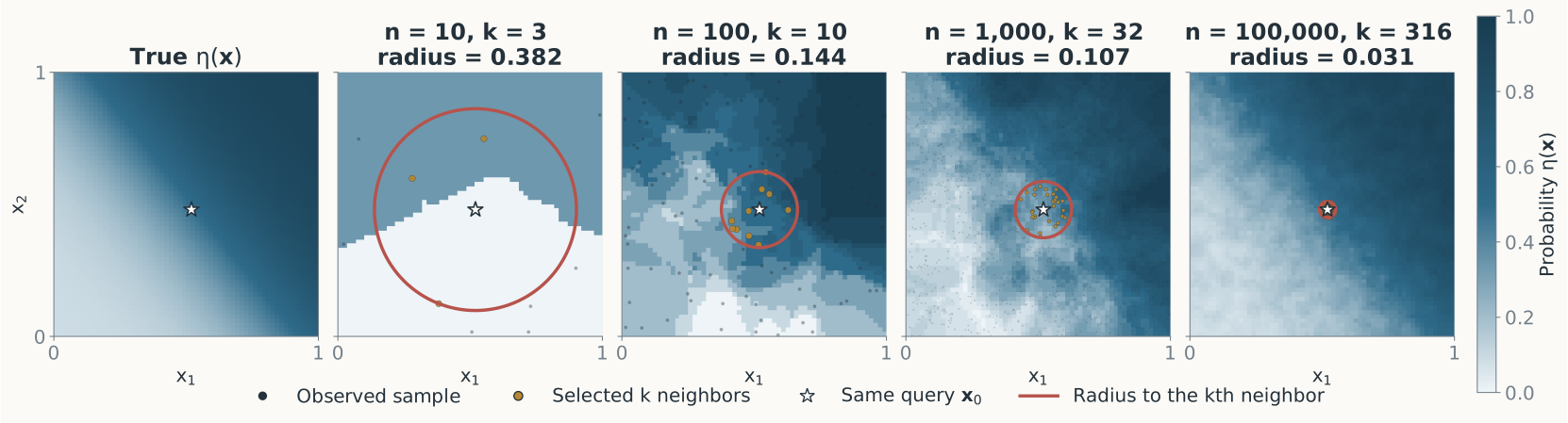
Here \(k=\lfloor\sqrt n\rfloor\), so \(k\to\infty\) while \(k/n\to0\): the same query averages more labels inside a smaller neighborhood.

[Sources] - source:stone-consistent-nonparametric-regression-1977

This is a controlled simulation with two abstract standardized coordinates, not an empirical bank result. The first panel is the ground-truth conditional probability. Each remaining panel shows a KNN probability estimate from a nested prefix of one sample sequence. Faint points are all observations, gold points are the k selected neighbors around the same starred query, and the red circle reaches the kth neighbor. The sqrt(n) schedule is illustrative: it satisfies the classic consistency direction but is not presented as universally optimal for a finite dataset. Increasing k reduces label noise; keeping k/n small allows the physical neighborhood to contract as the sample becomes dense. Stone’s result is much broader than this visualization; do not present a proof.

Smooth local structure is easier to estimate with finite data

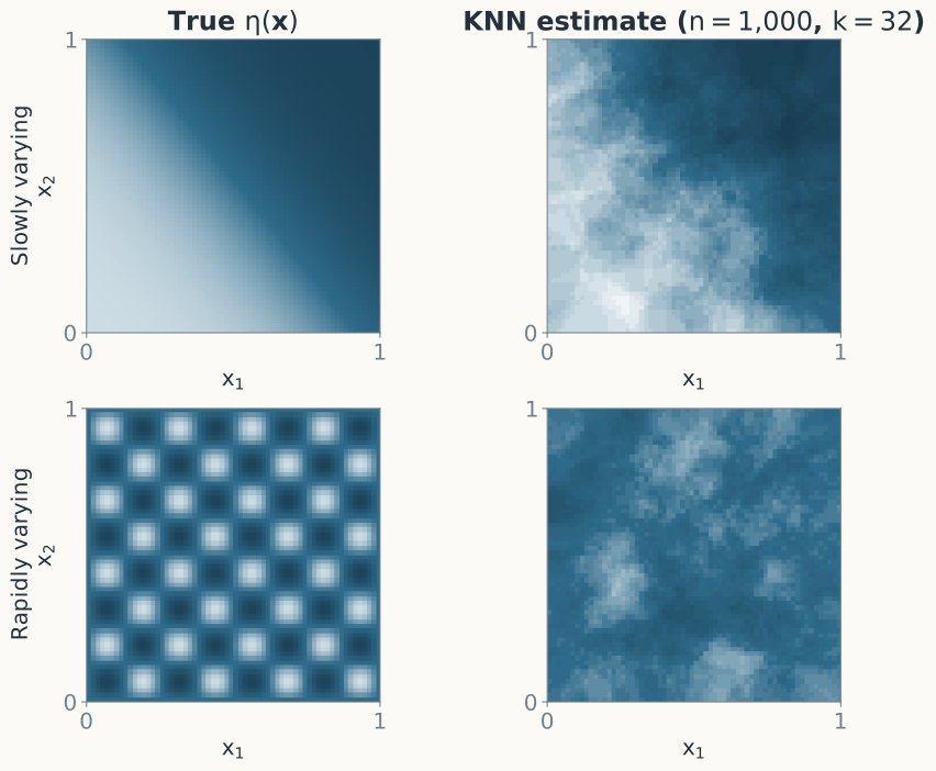
Local averaging recovers slowly varying probabilities sooner. Fine-scale or choppy structure can remain blurred until the sample is extraordinarily dense.

This is a finite-sample intuition, not an assertion that differentiability is required for every asymptotic consistency theorem. The lower response surface oscillates rapidly. With n=1,000 and k=32, each neighborhood averages across several changes in probability. The figure is generated by the same deterministic script as the growing-data illustration.

KNN defers nearly all computation until prediction

def fit(X, y):
    return np.asarray(X, float), np.asarray(y)

def predict_proba(model, X_new, k):
    X, y = model
    d2 = ((X_new[:, None, :] - X[None, :, :])**2).sum(2)
    nbr = np.argpartition(d2, k - 1, axis=1)[:, :k]
    return y[nbr].mean(axis=1)

Fit

• no parameter optimization
• store \(n\times d\) inputs and \(n\) labels
• memory and copy: \(O(nd)\)

Predict one input

• compute all \(n\) distances
• partial selection avoids a full sort
• time: \(O(nd)\)

Small reference sets can be cheap; very large ones motivate models that compress training evidence into learned parameters.

This is intentionally one efficient illustrative implementation, not a survey of trees, approximate search, batching, or production libraries. np.argpartition avoids sorting all n distances. A fully vectorized batch materializes a queries-by-training matrix, so large applications batch the queries. Say that fit has no optimization, not literally zero work: data still must be validated, transformed, and stored. Preview parametric linear and deep models without teaching them here. The dimensionality problem returns near the end of the arc.

3. Why can fitting the examples mislead us?

Observed success may reflect memorization, sample luck, or the wrong flexibility.

Training accuracy cannot tell us which \(k\) predicts best

Training accuracy on 3,000 distinct records from the bank use case:

\(k\)	1	25	151
Training accuracy	100.0%	90.1%	89.7%

Which value of \(k\) will give us the best predictions?

A. \(k=1\), because its training accuracy is highest.

B. \(k=25\), because it balances local detail and averaging.

C. \(k=151\), because it averages the most neighbors.

None of them. Training accuracy does not tell us which value predicts unseen customers best. We need different evidence.

Live multiple choice, about two minutes. Poll before revealing the intentional “none of them” twist. Training accuracy measures reuse of fitted records, not prediction on unseen customers. A is deliberately tempting because k=1 memorizes each distinct training input. B and C offer plausible intuitions about smoothing, but these measurements do not justify either one. One of the three values may in fact predict unseen customers best; the point is that training accuracy cannot identify it. This creates the need for held-out evidence on the next slide.

[Sources] - source:uci-bank-marketing-data

The values use a deterministic 3,000-row sample from the archived UCI Bank Marketing data after removing duplicate pre-call input rows. Duration and the outcome are excluded from the inputs. Numeric attributes are standardized; categorical attributes are one-hot encoded. The three KNN models are then scored on those same 3,000 fitted records. These are real training accuracies for this specified preprocessing and sample, not claims about unseen performance.

Training error answers an easier question

Quantity	Examples being scored	Question answered
Training error	Used to construct \(f\)	How well does \(f\) reproduce evidence it already saw?
Population error \(R_p(f)\)	Unseen draws from \(p\)	How often will \(f\) fail on the cases we care about?

The same observations cannot simultaneously serve as unrestricted construction material and untouched evidence of generalization.

Return to the population objective from the opening. The problem is not that training error is computed incorrectly; it answers a different, easier question. KNN makes the mismatch especially visible, but the distinction applies to every learned predictor.

A holdout lets observed data play the role of unseen data

We do not have outcomes for the genuinely unseen customers we ultimately care about. How can we estimate their error?

\[ \underbrace{\mathcal D_{\mathrm{train}}}_{\text{construct }f} \qquad\Big|\qquad \underbrace{\mathcal D_{\mathrm{holdout}}}_{\text{pretend unseen; score once}} \]

Reserve some observed pairs before fitting. Because their outcomes did not help construct \(f\), predictions on them mimic the information boundary of an unseen case—under the same sampling assumptions.

Lead with the question, pause briefly, then give the simple answer: act as though some observed examples are unseen by withholding them during training. The connection is informational, not temporal; the holdout may consist of historical rows. This is a development holdout at this stage, not yet a final test set. The i.i.d. assumption is what connects its errors to the target population.

Cross-validation rotates which fold is held out

Split one observed dataset into folds. Each fold takes one turn as untouched evaluation data.

	Fold 1	Fold 2	Fold 3	Fold 4	Fold 5
Fit 1	score \(e_1\)	train	train	train	train
Fit 2	train	score \(e_2\)	train	train	train
Fit 3	train	train	score \(e_3\)	train	train
Fit 4	train	train	train	score \(e_4\)	train
Fit 5	train	train	train	train	score \(e_5\)

\(K\) fits produce \(K\) errors, then we average: \(\widehat R_{\mathrm{CV}}=\frac1K\sum_{j=1}^{K}e_j\)

Leave-one-out cross-validation is the small-data extreme: \(K=n\).

The five-column bar is one dataset, not five separately collected datasets. Five or ten folds are common, but do not present either as universally best. Fit scaling and every learned preprocessing step inside each training fold. The fold errors are correlated because the training sets overlap, so CV does not create K independent experiments. CV is less central in many modern large-data workflows, but students should know the term and computational structure. About three minutes.

The neighbor count controls how much local detail survives

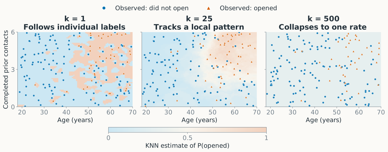
\(k=1\) can overfit individual outcomes; using every example erases useful local structure. Held-out error can reveal both failures.

This slide begins the flexibility question after cross-validation completes the held-out-evaluation idea. The illustration uses a controlled response simulation with plausible bank-case coordinates, not an empirical result from the UCI Bank Marketing data. Small k preserves sample noise, intermediate k borrows local evidence, and k=n underfits by returning the global positive rate everywhere. Do not claim that k=25 is optimal outside this illustration.

Bias compares the average fitted estimate with the target relationship

At one fixed test point \(\boldsymbol{x}\), imagine refitting the method on many possible training samples. Their average prediction is where the method tends to land:

\[ \mu(\boldsymbol{x}) =\mathbb E_{\mathcal D}\!\left[\widehat\eta_{\mathcal D}(\boldsymbol{x})\right], \qquad \operatorname{Bias}(\boldsymbol{x}) =\mu(\boldsymbol{x})-\eta(\boldsymbol{x}). \]

Real data lets us observe how estimates vary across samples. It does not reveal the true \(\eta(\boldsymbol{x})\), so formal bias remains unknown.

Bias is a property of a learning procedure across possible training samples, not merely one fitted model’s visible error. Keep the discussion at one fixed test point. Real observations do not reveal eta, so the later empirical figure can illustrate sample sensitivity but cannot measure formal bias.

Bias measures offset; variance measures spread

At age 40 (the only feature), each blue dot uses a different disjoint training set \(\mathcal D\) of \(n=1{,}647\) or \(1{,}648\) records. Each row reuses the same 25 sets.

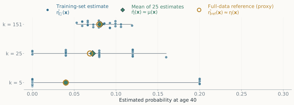
\[ \operatorname{Bias}(\boldsymbol{x}) ={\color{#3f7f6b}\mu(\boldsymbol{x})} -{\color{#b8872f}\eta(\boldsymbol{x})} \]

\[ \operatorname{Var}_{\mathcal D}\!\left({\color{#2f6b8a}\widehat\eta_{\mathcal D}(\boldsymbol{x})}\right) =\mathbb E_{\mathcal D}\!\left[ \left({\color{#2f6b8a}\widehat\eta_{\mathcal D}(\boldsymbol{x})} -{\color{#3f7f6b}\mu(\boldsymbol{x})}\right)^2\right] \]

True \(\eta\) is unknown: the diamond-to-ring gap is a bias proxy. The reference may itself be biased.

[Sources] - source:uci-bank-marketing-data

The 41,188 archived bank records are randomly partitioned into 25 disjoint training datasets: 13 contain 1,648 records and 12 contain 1,647. Each fit trains on one subset, unlike cross-validation, which trains on the complement of a held-out fold. All three rows reuse the same subsets and the same fixed query, age 40, with age as the only feature. Within each subset, the estimate averages the outcomes of its k nearest neighbors; n is the training-set size, not k. Diamonds mark the mean of the 25 estimates, an empirical approximation to mu. Gold rings are full-data reference fits using approximately the same neighbor fraction (25k neighbors). Neither marker is the unknown true eta. The empirical spread illustrates the theoretical variance over possible training samples; the finite partition does not measure that population quantity exactly. The diamond-to-ring difference is only an illustrative bias proxy. Because the reference uses the same neighbor fraction, it can share the small-sample fits’ smoothing bias. A small gap therefore does not establish small true bias. The approximation to eta in the legend is a working proxy, not a verified claim of accuracy. The equations define population bias and variance; the plotted mean and spread approximate their corresponding expectations over training samples. Vertical offsets only separate dots for readability. Discrete stacks occur because each estimate is an average of binary labels. A wider neighborhood may increase bias even when it reduces sample sensitivity.

Expected squared error combines bias, variance, and label noise

Draw a new input \(\mathbf{x}\) and binary outcome \(\textnormal{y}\) from the target population, independently of the training set \(\mathcal D\). How far is the predicted probability from the actual outcome, averaged over new cases and refits?

\[ \begin{gathered} \underbrace{\mathbb E_{\mathcal D,\mathbf{x},\textnormal{y}} \left[(\widehat\eta_{\mathcal D}(\mathbf{x})-\textnormal{y})^2\right]} _{\text{expected squared prediction error}} \\[0.6em] =\mathbb E_{\mathbf{x}}\!\left[ \underbrace{\operatorname{Bias}(\mathbf{x})^2}_{\text{systematic mismatch}} + \underbrace{\operatorname{Var}_{\mathcal D}(\widehat\eta_{\mathcal D}(\mathbf{x}))}_{\text{sample sensitivity}} + \underbrace{\eta(\mathbf{x})(1-\eta(\mathbf{x}))}_{\text{unresolved outcome variation}} \right]. \end{gathered} \]

Squared error loss gives this exact sum. Modeling choices can trade bias against variance; the represented inputs determine the remaining outcome noise.

This is squared error for probability estimation, not a decomposition of 0-1 classification error or accuracy. Explain the three terms intuitively before the following slides derive the identity by first conditioning on a fixed input and then averaging over the input distribution. Both x and y are random here; their joint distribution allows y to depend on x. Only the new pair is independent of the training dataset. Keep the label-noise term subordinate: the main instructional contrast is systematic mismatch versus sensitivity to the sampled training data.

Centering the outcome at \(\eta\) separates estimation error and noise

Fix \(\boldsymbol{x}\). Write \(\widehat\eta_{\mathcal D}=\widehat\eta_{\mathcal D}(\boldsymbol{x})\) and \(\eta=\mathbb E[\textnormal{y}\mid\boldsymbol{x}]\). The new outcome is independent of the training set given this input.

\(\displaystyle \mathbb E_{\mathcal D,\textnormal{y}}[(\widehat\eta_{\mathcal D}-\textnormal{y})^2\mid\boldsymbol{x}]\)

\(=\)

\(\displaystyle \mathbb E_{\mathcal D,\textnormal{y}}[((\widehat\eta_{\mathcal D}-\eta)+(\eta-\textnormal{y}))^2\mid\boldsymbol{x}]\)

(Add and subtract \(\eta\))

\(=\)

\(\displaystyle \begin{aligned}[t]&\mathbb E_{\mathcal D}[(\widehat\eta_{\mathcal D}-\eta)^2]+\mathbb E_{\textnormal{y}}[(\eta-\textnormal{y})^2\mid\boldsymbol{x}]\\&\quad+2\mathbb E_{\mathcal D}[\widehat\eta_{\mathcal D}-\eta]\,\underbrace{\mathbb E_{\textnormal{y}}[\eta-\textnormal{y}\mid\boldsymbol{x}]}_{\eta-\mathbb E[\textnormal{y}\mid\boldsymbol{x}]=\eta-\eta=0}\end{aligned}\)

(Expand; independence factors the cross term, and centering makes it zero)

\(=\)

\(\displaystyle \mathbb E_{\mathcal D}[(\widehat\eta_{\mathcal D}-\eta)^2]+\underbrace{\mathbb E[\textnormal{y}^2\mid\boldsymbol{x}]-\eta^2}_{\operatorname{Var}(\textnormal{y}\mid\boldsymbol{x})}\)

(Expand the remaining outcome square)

\(=\)

\(\displaystyle \underbrace{\mathbb E_{\mathcal D}[(\widehat\eta_{\mathcal D}-\eta)^2]}_{\text{probability-estimation error}}+\underbrace{\eta(1-\eta)}_{\text{outcome noise}}\)

(Binary \(\textnormal{y}^2=\textnormal{y}\), so \(\eta-\eta^2=\eta(1-\eta)\))

The starting expression is squared prediction error against a new outcome at a fixed input. Each subsequent equality is one reveal; the expanded square and its zero cross term appear together. Conditional independence of the new outcome and D factors that cross term. Its outcome factor is zero because eta is the conditional mean. Expanding the remaining outcome square gives E[y squared | x] - 2 eta E[y | x] + eta squared, hence E[y squared | x] - eta squared. For a binary outcome, y squared equals y. Conditioning on bold italic x abbreviates random bold upright x equals this fixed input. D-only expectations need no conditioning bar because the new input and training dataset are independent. Every fit is still evaluated at this x. This intermediate expression separates error in estimating the probability from outcome noise; the next slide decomposes the estimation error. Allow five to six minutes, including student questions about the cross term.

Centering the fit at \(\mu\) separates squared bias and variance

At the same fixed \(\boldsymbol{x}\), let \(\mu=\mathbb E_{\mathcal D}[\widehat\eta_{\mathcal D}]\). Continue from the preceding slide, keeping its outcome-noise term.

\(\displaystyle \mathbb E_{\mathcal D}[(\widehat\eta_{\mathcal D}-\eta)^2]+\eta(1-\eta)\)

\(=\)

\(\displaystyle \mathbb E_{\mathcal D}[((\widehat\eta_{\mathcal D}-\mu)+(\mu-\eta))^2]+\eta(1-\eta)\)

(Add and subtract \(\mu\))

\(=\)

\(\displaystyle \begin{aligned}[t]&\mathbb E_{\mathcal D}[(\widehat\eta_{\mathcal D}-\mu)^2]+(\mu-\eta)^2+\eta(1-\eta)\\&\quad+2(\mu-\eta)\,\underbrace{\mathbb E_{\mathcal D}[\widehat\eta_{\mathcal D}-\mu]}_{\mathbb E_{\mathcal D}[\widehat\eta_{\mathcal D}]-\mu=\mu-\mu=0}\end{aligned}\)

(Expand; \(\mu-\eta\) is constant across training sets, and the centered fit has mean zero)

\(=\)

\(\displaystyle \underbrace{(\mu-\eta)^2}_{\text{squared bias}}+\underbrace{\mathbb E_{\mathcal D}[(\widehat\eta_{\mathcal D}-\mu)^2]}_{\text{variance}}+\underbrace{\eta(1-\eta)}_{\text{outcome noise}}\)

(The cross term is zero; reorder the remaining terms)

This exact sum uses squared error loss. Other losses need different analyses.

Continue the same equality chain from the preceding slide. The expanded square and the explanation of its zero cross term are one reveal, not a later aside. Mu and eta depend on the fixed input but do not vary across D, so pull mu minus eta outside the expectation. The remaining factor is zero by the definition of mu. No independence between hat_eta_D and its own deviation is assumed. Bias is where the procedure tends to land relative to the true probability; variance is how much it moves when its training sample changes. Noise remains even at the true probability. The learning procedure and sample size are fixed across refits. The next slide averages the pointwise identity over inputs to recover the population formula. Allow five to six minutes, including discussion of why mu minus eta is constant across training datasets.

Averaging over inputs gives population squared prediction error

Now draw a new input \(\mathbf{x}\) from the target population and its outcome \(\textnormal{y}\). Average the pointwise identity over those inputs:

\[ \begin{gathered} \underbrace{\mathbb E_{\mathcal D,\mathbf{x},\textnormal{y}} [(\widehat\eta_{\mathcal D}(\mathbf{x})-\textnormal{y})^2]}_{\text{average error on new cases, across refits}} \\[0.6em] =\underbrace{\mathbb E_{\mathbf{x}}[\operatorname{Bias}(\mathbf{x})^2]}_{\text{average squared bias}} +\underbrace{\mathbb E_{\mathbf{x}}[\operatorname{Var}_{\mathcal D}(\widehat\eta_{\mathcal D}(\mathbf{x}))]}_{\text{average variance}} +\underbrace{\mathbb E_{\mathbf{x}}[\eta(\mathbf{x})(1-\eta(\mathbf{x}))]}_{\text{average outcome noise}}. \end{gathered} \]

• Inputs count according to how often they occur in the target population. The decomposition stays exact, but its terms now summarize all inputs.
• Average squared bias: positive and negative biases at different inputs cannot cancel each other.

Why it matters: smoothing can reduce sample sensitivity while increasing systematic mismatch. Held-out error measures their combined effect, plus outcome noise.

The left-hand side averages over both hypothetical refits and independent new test cases. It describes the learning procedure at a fixed sample size, rather than the risk of one particular fitted model. For one realized dataset D, test risk averages only over x and y; the displayed decomposition holds after also averaging over D. For probability estimation against eta instead of a realized outcome, omit the noise term on both the pointwise and population versions. Linearity of expectation preserves the three-term sum without extra cross terms. E_x[Bias(x)^2] is not (E_x[Bias(x)])^2. Local failures can still be hidden by a population average, particularly for rare inputs. The noise is unresolved given the represented inputs, not necessarily irreducible under richer features. Real held-out labels estimate total prediction error, not these separate unknown components. This explains why knowing that k reduces variance does not by itself tell us which k gives the best predictions. About three minutes.

Increasing \(k\) exchanges local detail for stability

Smaller \(k\)	Larger \(k\)
uses closer evidence	reaches farther from the query
follows more sample-specific detail	averages more observed outcomes
often lower local bias, higher variance	often higher local bias, lower variance

Neither extreme is automatically best. Held-out error measures the combined effect for the population and representation we care about.

Use “often” deliberately. Actual bias, variance, and classification error need not change monotonically with k. Reconnect the table to the flexibility figure and the real-data sampling variation rather than introducing a generic U-shaped cartoon as fact.

Data and representation improve the same local-evidence mechanism

Change	What happens to a KNN neighborhood?
More representative training data	genuinely similar examples can be closer
Better scaling or features	distance favors differences relevant to the outcome
Larger \(k\)	more outcomes are averaged, but evidence comes from farther away

All three change the evidence inside \(\widehat\eta_k(\boldsymbol{x})\) and therefore its bias and variance.

This synthesis closes Question 3. More data does not automatically help if it comes from the wrong population, and better representation does not remove the need for evaluation. The next question asks how held-out evidence changes once we use it to choose among alternatives.

4. How can we choose a model without fooling ourselves?

Choosing a predictor and measuring its performance are two different uses of data.

Which neighbor count should we choose?

We fit KNN with \(k=1,5,25\) and choose the lowest training error. Inputs are distinct, and each training point counts as its own neighbor.

Is this a reliable way to choose the best predictor for new cases?

A. Yes: evaluating every candidate on the same examples makes the comparison fair.

B. No: training error rewards reproducing outcomes the predictor already used.

C. No: we should always choose the largest \(k\) to get the most stable predictions.

B. Here, \(k=1\) gets zero training error by retrieving each point’s own label. That does not establish how well it predicts a new outcome.

Live retrieval check, about two minutes. The setup ensures the self-neighbor argument is exact, avoiding conflicting labels at duplicate inputs. Same-data comparison does not fix the reuse of training labels. C confuses stability with overall prediction quality: excessive smoothing can introduce bias. Reconnect to the earlier training-versus-population error distinction before introducing validation as the appropriate evidence for choosing k.

A held-out validation set lets us compare candidate values of \(k\)

Fit each candidate using \(\mathcal D_{\mathrm{train}}\). Evaluate its predictions on the same separate \(\mathcal D_{\mathrm{validation}}\), then choose the lowest validation error.

\[ \mathcal D_{\mathrm{train}} \xrightarrow{\ \text{fit}\ } f_1,f_5,f_{25} \xrightarrow{\ \text{score on validation}\ } \widehat k=\arg\min_{k\in\{1,5,25\}}\widehat R_{\mathrm{validation}}(f_k). \]

The validation outcomes are unavailable when fitting each candidate. They give us evidence about prediction on cases outside that candidate’s training set.

About two minutes. Validation is the appropriate role for choosing k. Candidates and their preprocessing are fitted using training data only. Under independent, representative sampling, each fixed candidate’s empirical validation error is unbiased for its population error. This does not make either the winning score or the selection decision “unbiased”; choosing the best true model remains uncertain with finite data. Defer that distinction to the next question. The errors in this section are 0–1 classification errors, not the squared probability errors used in the preceding bias–variance identity.

What does the selected model’s 4.5% error tell us?

We choose \(k\) with the lowest validation error and report its 4.5% as the selected model’s estimated population error.

Across repetitions of this procedure, is the reported error lower on average, unbiased, or higher on average?

A. Lower than the selected model’s true population error on average.

B. Unbiased for the selected model’s true population error.

C. Higher than the selected model’s true population error on average.

A: optimistic selection bias. Choosing the lowest observed error also favors favorable validation noise. Validation appropriately helps choose \(k\), but the winning score is no longer an unbiased final evaluation.

Live multiple choice, about three minutes. The 4.5% is an illustrative scenario, not a measured result from the bank dataset. Compare each selected model’s validation error with that same model’s true population error, then average over repetitions. Fixed candidates may each have unbiased validation scores, yet choosing the minimum introduces downward selection bias. Correlations among candidate scores and the number of choices affect its magnitude. The bias can be zero in degenerate cases; never claim that every observed validation error must be below its population error. A particular selected model may truly have population error below 4.5%. Nor is selecting k guaranteed to find the population optimum. The method is appropriate for selection, while reuse of its winning score as a final estimate creates the problem. Error optimism corresponds to accuracy optimism in the opposite direction: 4.5% error is 95.5% accuracy.

Validation is held out of each fit, but participates in selection

What are we evaluating?	Did validation outcomes help construct it?
One candidate fitted at a fixed \(k\)	No: only the training data determined that fit.
The selected pipeline, including the choice of \(k\)	Yes: validation errors determined which candidate won.

Selection is part of learning. Information from validation enters through our choice of \(k\), even though the KNN fitting step never reads those labels.

The same reuse occurs when validation guides features, preprocessing, or model families. It leaks into a claimed final evaluation through those choices.

About three minutes. This is indirect information reuse, distinct from scoring on the very rows used for fitting. It can be much subtler than training-set reuse, but do not promise it is always small: extensive adaptive searching can severely overfit validation data. Using validation to select is intentional and appropriate; treating its selected score as untouched final evidence is the mistake. Human error inspection and AI-driven iteration also belong to the selection process when they influence the final pipeline. For this reason the information boundary must surround the full process, not just model.fit().

Separate validation for choosing from test data for reporting

Reserve all three roles before development:

Data	Role	What may it influence?
Training	Fit each candidate.	Its learned parameters or stored examples.
Validation	Compare candidates and choose \(k\).	The selected pipeline.
Test	Score the settled pipeline once.	The reported performance estimate.

Freeze the pipeline before using the test outcomes. An independent, representative test set gives an unbiased error estimate for that fixed pipeline, with finite-sample uncertainty.

About three minutes. If refitting on training plus validation data after selecting k, complete that refit before opening the test set; the test evaluates that refitted predictor. Fit any learned preprocessing within the permitted fitting data. Do not change the pipeline in response to test performance and retain the same claim of untouched evaluation. Cross-validation can rotate the validation role within development data, but a final independent test role is still needed for an honest final estimate after selection. This slide resolves both earlier questions: training fits, validation chooses, and test evaluates the result of the whole development process. An unbiased estimate can still be noisy or unrepresentative of deployment if the sampling assumptions fail.

Refit the chosen pipeline before opening the test set

After choosing \(k\) and all other pipeline settings, we may fit once more on training + validation data to use all development examples.

\[ \underbrace{\mathcal D_{\mathrm{train}}\cup\mathcal D_{\mathrm{validation}}}_{\text{refit with settled choices}} \quad\longrightarrow\quad f_{\mathrm{final}} \quad\xrightarrow{\ \mathcal D_{\mathrm{test}}\ }\quad \widehat R_{\mathrm{test}}(f_{\mathrm{final}}). \]

For KNN, this means storing all development examples with the chosen \(k\) and refitting any learned preprocessing on those development examples.

The test result describes this final predictor. Changing it after seeing the test result turns that test into more development evidence.

About three minutes. Refit is optional, but the order matters. More development examples can change the learned predictor even when its settings stay fixed. Thus the earlier winning validation score does not directly score the refitted predictor. The untouched test set does. Decide the refitting procedure before opening the test set. This does not guarantee that refitting always improves performance or that the k selected on smaller fits remains optimal. If test results motivate further changes, acknowledge renewed development and obtain fresh independent evidence before making another untouched-evaluation claim.

Keep final testing outside every development feedback loop

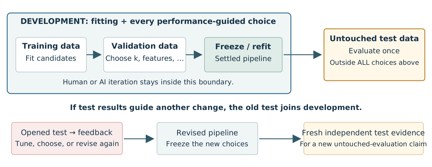
One final test can cover all development choices. A new split is needed when we reuse final-test feedback to make further choices—not for every fitting step.

About two minutes. This makes the information boundary visible. The test must remain outside preprocessing, hyperparameter selection, feature decisions, and human or AI error-driven iteration. Independent representative testing gives an unbiased estimate for the fixed evaluated pipeline; it does not remove sampling uncertainty or population mismatch. Merely observing a test score does not force a new split if the model remains fixed. Reusing its outcomes to select a revision does change its role. CV remains in the previously delivered introductory slide; this continuation uses only train/validation/test. Next: what can the resulting score tell us about real deployment?

5. When and why should a learned solution hold?

A test score becomes useful when we understand its uncertainty and the scope of its evidence.

Interpret the score through three connected questions

Our reasoning process	Question to resolve
1. What did the test measure? ← now	How much evidence is behind this score?
2. Does it represent deployment?	Could dependence, population, or available information differ?
3. What can we claim?	State the supported result and the conditions for extending it.

We protected the test from selection. Now interpret what it tells us.

Brief orientation. No PAC-style guarantee unit here. The point is to distinguish an honest but finite measurement from a claim about future deployment.

A rough 95% interval is the score ± two standard errors

Fix the model before testing on \(m\) independent examples from the target population. Let \(\widehat a\) be the fraction of test predictions that are correct.

\[ \text{Approximate 95\% interval:}\qquad \widehat a\ \pm\ 2\sqrt{\frac{\widehat a(1-\widehat a)}{m}}. \]

900 correct out of 1,000: 90% accuracy, with a margin of about 1.9 percentage points.

“With approximately 95% confidence, this fixed model’s accuracy in this population is between 88% and 92%.”

About two minutes. [Sources] source:nist-binomial-confidence-intervals. Accuracy is an average of independent Bernoulli correct/incorrect indicators. Its estimated standard error is sqrt(a_hat(1-a_hat)/m); 1.96 is the usual normal 95% multiplier, rounded to 2. At 900/1000 the two-standard-error margin is 1.897 percentage points, so the displayed whole-percent sentence is deliberately rough. If repeated independent test samples were used to build these intervals, roughly 95% would cover the fixed population accuracy under the approximation. This is not a 95% probability for each prediction or a guarantee for a new population. A common rough adequacy check is at least ten correct and ten incorrect outcomes; near 0%/100% or at small m, use Wilson (examples in notes), not a zero-width Wald interval. This formula is for ordinary accuracy or binary error rate, not directly for balanced accuracy, F1, AUC, subgroup comparisons, or dependent windows. No PAC learning statement or epsilon/delta formalism. Hold the model and population fixed.

A rough normal approximation: use Wilson intervals for small samples or few errors. This measures finite-test uncertainty, not protection against leakage or distribution shift.

More test examples support more precise claims

Suppose measured accuracy is 90% in each case:

Independent test examples	Correct predictions	Rough 95% margin (pp)
10	9/10 = 90%	±19†
30	27/30 = 90%	±11†
100	90/100 = 90%	±6
1,000	900/1,000 = 90%	±1.9
2,000	1,800/2,000 = 90%	±1.3
5,000	4,500/5,000 = 90%	±0.8
10,000	9,000/10,000 = 90%	±0.6

10–30: wide uncertainty. 1,000–10,000: roughly 2-point to sub-1-point precision here.

About two minutes. [Sources] source:nist-binomial-confidence-intervals. Displayed margins are 100 × 2sqrt(.9 × .1 / m), rounded: 18.97, 10.95, 6.00, 1.90, 1.34, 0.85, 0.60 percentage points (m=10,30,100,1000,2000,5000,10000). These are normal-approximation scales, not Wilson half-widths. At m=10 or 30 there are too few errors for reliable normal coverage; the dagger explicitly marks those rows. Do not interpret 90% ±19 points as a valid interval or simply clip it at 100%. For actual small-sample intervals, Wilson gives 59.6%–98.2% for 9/10 and 74.4%–96.5% for 27/30 (z=1.959963984540054). For m=10, even nine correct predictions supports only about 60%–98% accuracy. At 1000 the interval is about 88.0%–91.7%; at 10000 about 89.4%–90.6%. Margin shrinks like 1/sqrt(m): ten times more precision needs 100 times more data. Emphasize practical percentage-point precision rather than decimal-place targets. Report the estimate with its margin and decide whether that precision is useful. For rare failures, subgroup scores, or high-stakes decisions, even 10000 may be insufficient. More same-population data cannot repair deployment mismatch.

pp = percentage points. Margins use the previous slide’s rough formula. †Small-sample scale only: use Wilson for an actual interval. Fixed model; independent, representative test examples.

Next ask whether the evidence matches deployment

Our reasoning process	What we have established
1. What did the test measure?	A count of errors from a finite sample.
2. Does it represent deployment? ← now	Check independence, population, and available information.
3. What can we claim?	Combine the measured result with the scope of its evidence.

A very large test set can measure the wrong deployment population very precisely.

About 30 seconds. Numbers are not meaningless when an assumption fails. Identify which inference needs that assumption and what weaker claim remains. This section traces assumptions to concrete failure modes and evaluation choices.

Repeated rows need not provide independent evidence

Imagine 100 customers, each represented by 10 related campaign records.

• A random row split may put the same customer in both training and test data.
• A model may exploit person-specific information that will not help on a new customer.
• The 1,000 rows also need not provide the precision of 1,000 independent customers.

If the claim concerns new customers, keep each customer in one split.

About two minutes. Hypothetical example, not a claim that UCI has verified customer IDs or precisely this duplication. Dependence does not necessarily bias every sample mean, but treating the rows as independent understates uncertainty. Effective sample size depends on dependence structure; do not declare it exactly 100. Shuffling rows does not make related observations independent. If deployment is future events for known people, the relevant design can differ.

Independent examples can still come from a different population

\[ R_p(f)=\Pr_{(\mathbf{x},\textnormal{y})\sim p}\{f(\mathbf{x})\ne\textnormal{y}\}, \qquad R_q(f)=\Pr_{(\mathbf{x},\textnormal{y})\sim q}\{f(\mathbf{x})\ne\textnormal{y}\}. \]

• The test set estimates performance under \(p\).
• Deployment may draw customers and outcomes from \(q\ne p\): distribution shift.
• Out-of-distribution (OOD) performance depends on \(q\); even perfect knowledge of \(R_p(f)\) does not determine \(R_q(f)\).

What changes operationally—and could it change who responds to our offer?

About two minutes. This breaks the identical-distribution link between evaluation and deployment even if each sample separately consists of independent examples. OOD here means a changed joint distribution, not necessarily feature values outside the observed range. Shift can change performance mildly, severely, or not at all; its effect depends on the model and the changed relationship.

Would this new contact list preserve accuracy?

Synthetic bank campaign: a frozen age-only KNN model is 90% accurate under the original list. A new supplier provides the same age distribution and same overall account-opening rate.

Do those checks establish similar accuracy on the new list?

A. Yes: the input distribution and overall outcome rate are unchanged.

B. No: the relationship between age and opening may have changed.

C. Yes, if we make the original-list test set much larger.

B. Matching the separate summaries does not establish a matching joint relationship.

About two minutes, one commitment and reveal. This is a deliberately constructed synthetic case; no empirical UCI result or typical effect size is claimed. The new supplier is operationally ordinary, not mathematically a small change. C tightens estimation of the old population instead of measuring the new one.

The unchanged predictor falls from 90% to 10% accuracy

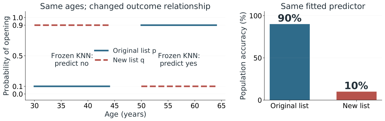
Synthetic bank example. Both lists: half ages 30–44, half ages 50–64; uniform ages within each group; 50% open overall. Only the relationship between age and outcome changes.

The old 90% remains valid for the old population. More old-list data cannot establish new-list accuracy.

About two minutes. Generated by lectures/scripts/arc3_shift_figure.py. Train once on 3,000 controlled source examples: 100 at each integer age, exactly 10% opening at each younger age and 90% at each older age. Fix k=101 and age as the only input; majority vote yields no for every younger age and yes for every older age. The generator evaluates exact population risks over 30 equally likely ages, not a tuned lucky test sample. Conditional probabilities reverse under q, so accuracy reverses exactly. The balanced 50% outcome rate is for clarity and is not the real bank dataset prevalence. The q outcomes are never used in fitting. A possible mechanism is a different mix of unobserved savings preferences within each age group. This is a hypothetical story, not a causal discovery: matching p(x) and p(y) does not establish matching p(x,y). No new age values are needed. The source-population result stays meaningful. Additional source test samples reduce sampling uncertainty, not the deployment gap. If useful at the board, write Rhat_p-R_q=(Rhat_p-R_p)+(R_p-R_q); the identity stays in notes rather than requiring another slide. This deliberately severe shift is not claimed typical.

Which test matches the claim about new people?

A walking classifier uses many sensor windows from each volunteer. Deployment will involve people absent from development data.

Which split most directly tests that claim?

A. Randomly assign windows to training and test sets.

B. Put each volunteer entirely in development or entirely in test.

C. Test later windows from volunteers already used for training.

B. It tests unseen people. It still does not establish transfer to different sensors, activities, or collection settings.

About two minutes. A transfer question using the smartphone-activity setting, source:uci-smartphone-activity. This is a hypothetical evaluation choice, not a new empirical result. A and C can support different claims about known people. Repeated windows within a test person remain correlated; grouping prevents person overlap but does not turn windows into independent people.

Choose the evaluation design from the deployment claim

Intended claim	More relevant evidence	What still needs reasoning?
More cases from the same population	Random held-out examples	Does the sample represent deployment?
Future campaigns	Train earlier, test on a later campaign	Will later changes resemble this one?
New customers	Keep each customer entirely in one split	Are these customers representative?

All designs require prediction-time inputs: current-call duration remains unavailable before the call. A split cannot repair that information mismatch.

About two minutes. No universally best split. Specify prediction unit, time, information, and intended population before choosing the design. Historical contacted clients do not automatically represent all potential customers. Chronological evaluation tests one observed transition, not every future shift. Changing a pipeline after inspecting a new-supplier test makes that data part of development; fresh final evidence is then needed for an untouched claim.

Finally state what the evidence supports

Our reasoning process	What we have established
1. What did the test measure?	Report the errors and number of test examples.
2. Does it represent deployment?	Examine dependence, changed populations, and available inputs.
3. What can we claim? ← now	State the supported result and the conditions for extending it.

A useful number comes with a reasoned account of where it applies.

Brief orientation, about 30 seconds. Return to the same three-stage roadmap. The next slide turns this framework into a concrete report with scope and uncertainty.

Report a result, its scope, and its uncertainty

Illustrative report: “The frozen before-call predictor made 100 errors on 1,000 independent held-out customers from supplier A’s campaign: 10% error.”

• Scope: one prediction per customer; account opening as the outcome; test data excluded from all development choices.
• Uncertainty: roughly 10% ±1.9 percentage points at 95% confidence.
• Extension: a different supplier may change response patterns within age groups. This result does not establish its error without evidence connecting the populations.

Say what may change, why it matters, and what evidence would resolve it.

About two minutes. These are hypothetical report counts, separate from the exact population-risk calculation in the shift illustration. The outcome and metric must also match the business goal; accuracy alone does not establish profit or causal benefit. More precise measurement for p is not a substitute for evaluating relevance to q.

From interpreting evidence to rethinking the predictor

So far: What does a settled model’s test score tell us about deployment?

Now: When does KNN’s notion of “nearby” stop being useful—and what should we learn instead?

Our next steps:

1. See how near and far distances become less distinct in high dimensions.
2. Test what happens when irrelevant features distort distance.
3. Motivate a learned score that emphasizes predictive information.

Brief section transition, about 30 seconds. Close Question 5’s interpretation argument explicitly. We now change the modeling question: even with trustworthy evaluation, raw locality can be a poor basis for prediction. This is the bridge from Arc 3 to Arc 4, not another evaluation caveat or an OOD-method discussion. The train/validation/test boundary still applies when comparing predictors.

In high dimensions, near and far become less distinct

Draw 500 points with independent standard-normal coordinates: \(\mathbf{x}_i\sim\mathcal N(\boldsymbol{0},\mathbf I_d)\). Plot every pairwise distance.

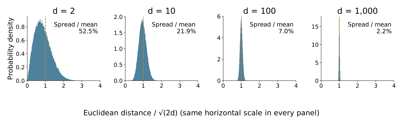
Typical raw distance grows like \(\sqrt{2d}\); its relative spread shrinks. Dividing by \(\sqrt{2d}\) lets us compare dimensions on the same scale.

A “near” point is only slightly closer than a “far” point: distance loses contrast.

About two minutes. [Sources] source:cornell-cs4780-knn-2018. The older illustration used independent uniform coordinates in a unit cube. This is a new reproducible Gaussian simulation, generated by lectures/scripts/arc3_distance_concentration.py. Use 500 points and nested independent coordinates at d=2,10,100,1000, seed20260928. All 124750 unordered pairs are shown, not just neighbors or distance to the origin. Pairwise distances share observations and are not independent replicates. All horizontal axes and histogram bin widths match; vertical density scales vary so each distribution’s width remains legible. The dashed line marks one. Spread means standard deviation; the reported coefficient of variation is unchanged by normalization. Normalizing every distance by the same dimension-dependent number does not change the neighbor ranking. For two independent standard Gaussian vectors, squared distance / 2 has a chi-square law with d degrees of freedom: squared distance has mean 2d and variance 8d. Thus distance / sqrt(2d) concentrates near one. Raw Euclidean distance’s absolute standard deviation approaches one; it does not shrink to zero. Avoid saying all points have exactly equal distances, or using central quantiles as nearest/farthest extremes. With a fixed finite sample, relative near/far contrast shrinks as d grows; very different sample-size growth or structured data can change the conclusion. This motivates the bank noise experiment; concentration alone does not prove classification must fail for every high-dimensional distribution or metric. The complementary sparse-coverage argument: a uniform-cube box of side r holds fraction r^d; holding r fixed requires exponentially many samples for fixed occupancy.

Add measurements that contain no new information

Return to our simulated bank campaign: age and prior contacts predict opening. Keep every customer and outcome fixed; append independent Gaussian columns.

\[ \boldsymbol{x}_{\mathrm{aug}}= [\,\text{age},\ \text{prior contacts},\ z_1,\ldots,z_d\,], \qquad \textnormal{z}_j\overset{\mathrm{iid}}{\sim}\mathcal N(0,1). \]

• Noise is independent of both the original features and the outcome.
• Standardize using training data; select \(k\) or regularization on validation.
• Same split: 500 training, 500 validation, 2,000 test customers.

Available predictive information is unchanged. Is distance still useful?

About two minutes. This is the original bank_flexibility simulation, not measured UCI bank data. Its nonlinear response law and seed 572 are unchanged. Append nested columns from one independent Gaussian draw with seed 20260928. Both methods get identical standardized features and class-balanced decisions. Every feasible k=1..500 is considered; L1 logistic C is selected from .001,.003,.01,.03,.1,.3,1. No split/seed search. The linear model is deliberately misspecified for the nonlinear bank law and need not beat KNN without noise.

Independent noise can make neighbors nearly uninformative

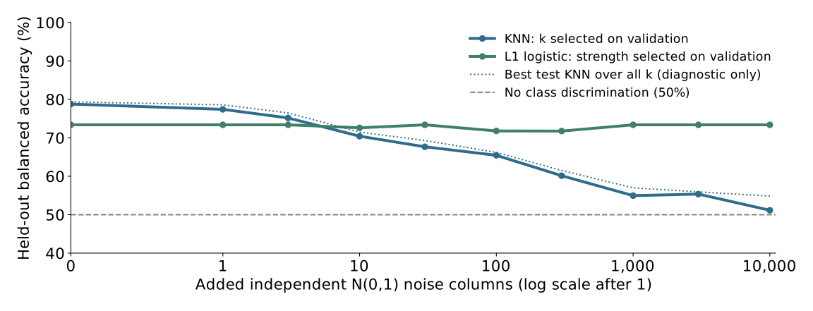
Balanced accuracy: average of the two class recall rates; 50% means no discrimination. At 10,000 noise columns: KNN 51.1%; learned-score model 73.4% (preview of Arc 4).

About two minutes. Generated by lectures/scripts/arc3_bank_noise.py, with exact results in bank-noise-results.json. Balanced accuracy prevents majority-class prediction from hiding failure in this imbalanced case. KNN uses a class-balanced vote (opening fraction greater than training opening prevalence); logistic uses balanced class weights. Both tune on validation balanced accuracy. The dotted curve is the diagnostic maximum test score across every feasible k, not a valid selection procedure: even that reaches only 54.8% with 10,000 noise columns. One fixed experiment, not an average over random repetitions or a universal rate. The endpoints are 78.8% to 51.1% KNN and 73.4% to 73.4% logistic. Regularization suppresses many noise coefficients; unregularized linear fitting is not promised this stability. The nonlinear response law explains the lower linear baseline.

Noise dominates distance; which coordinates should matter?

\[ \|\boldsymbol{x}_{\mathrm{aug}}-\boldsymbol{x}'_{\mathrm{aug}}\|^2 =\underbrace{\|\boldsymbol{x}_{\mathrm{signal}}-\boldsymbol{x}'_{\mathrm{signal}}\|^2}_{\text{two relevant coordinates}} +\underbrace{\sum_{j=1}^{d}(z_j-z'_j)^2}_{\text{many irrelevant coordinates}}. \]

• Independent noise differences accumulate and scramble which customers are nearest.
• Increasing \(k\) averages more labels; it does not identify the relevant coordinates.
• Could we learn which coordinates matter, giving irrelevant ones less influence?

High dimension alone is not the verdict: correlated features can carry redundant, useful structure. Real data need not fill the whole ambient space.

About two minutes. Linear models have not yet been taught. Pose learned feature importance as the next idea; do not assume knowledge of linear scores or penalties. Before finite-sample standardization, two independent standard normal vectors contribute a noise sum with mean 2d and standard deviation sqrt(8d). Relative distances concentrate, while absolute nuisance fluctuations grow and can overwhelm bounded signal differences. Raw Euclidean KNN gives all standardized coordinates equal weight. This experiment demonstrates that failure mechanism, not a theorem that every metric or representation must fail. Sparse regularization uses supervised evidence; with more noise and insufficient data it too can fail. The next real example tests the nuance. Correlation or lower intrinsic dimension can help, but neither guarantees a good distance nor is measured for this corpus.

Real-world example: movie-review sentiment

• 2,000 real reviews: predict positive or negative sentiment.
• 18,746 vocabulary words: represent each review with one numerical feature per word.
• Shared words need not mean shared sentiment: “good” versus “not good.”

A new idea: learn a positive or negative score for each word and combine the contributions. This leads to a linear model, which we will study next.

About one minute. [Sources] source:cornell-movie-review-polarity-v2 and source:cornell-movie-review-polarity-v2-data. This is an introduction and motivation, not a lesson on linear models or text preprocessing. Do not discuss TF–IDF here. Distinguish the review’s numerical word features from the word contributions a supervised model will learn. The exact representation and comparison protocol remain documented in the next slide’s notes and the reproducible script. “Good” and “not good” are instructor-created phrases, not corpus quotations. They illustrate that lexical overlap is not sentiment equivalence. Do not imply that independent word scores fully resolve negation or word order; the measured unigram model also has those limitations. A learned score is a promising change of predictor, not a solution to every language phenomenon. Real text has structure; high ambient dimension alone does not force chance-level KNN performance.

On real reviews, a learned score outperforms every tested \(k\)

Cornell movie reviews: positive versus negative sentiment; 18,746 word features. Train: 1,200 reviews; validate: 400; test: 400. No synthetic examples or added noise.

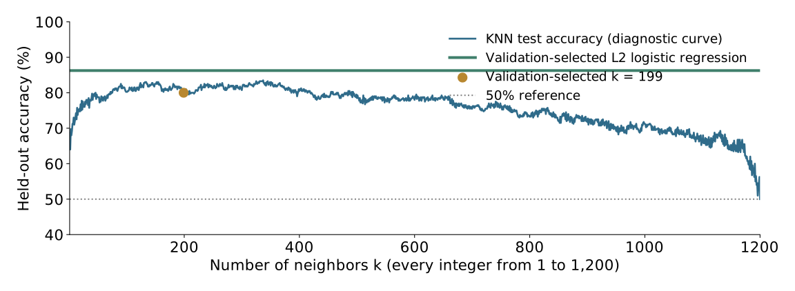
Validation-selected test accuracy: KNN 80.0%; learned word-score model 86.25%. Meaningful word features are not independent noise: KNN still has useful predictive signal.

About two minutes. The logistic regression curve previews the model family we will teach next; students need not know its training rule yet. Sources: source:cornell-movie-review-polarity-v2 and source:cornell-movie-review-polarity-v2-data. Original polarity v2.0, Pang and Lee, 2004. Fixed supplied filename folds cv0–5 train, cv6–7 validation, cv8–9 test; each split is class balanced. No split or seed search. Training-only unigram TF–IDF with min_df=2, sublinear_tf=True, norm=l2. Identical representation for both methods. KNN uses Euclidean distance, every k=1..1200, ties to negative; validation chooses k=199. L2 logistic selects C=100 from .01,.1,1,10,100 on validation. The test curve is diagnostic; test outcomes do not select hyperparameters. Correct counts are 320/400 versus 345/400; diagnostic best KNN is 334/400. This one split does not establish statistical superiority for all samples or prove dimensionality alone caused the gap. Labels derive from extracted ratings; the README warns unrecognized rating mentions can remain. This is within-corpus document evaluation, not author/movie/time-disjoint generalization or a guarantee for modern user reviews. Do not describe it as catastrophic KNN failure.

A useful one-dimensional projection separates the outcomes

\[ \boldsymbol{x}\in\mathbb R^{18746} \quad\longrightarrow\quad z=\boldsymbol{w}^{\mathsf T}\boldsymbol{x}+b\in\mathbb R \quad\longrightarrow\quad \widehat y=\mathbf 1\{z\ge0\}. \]

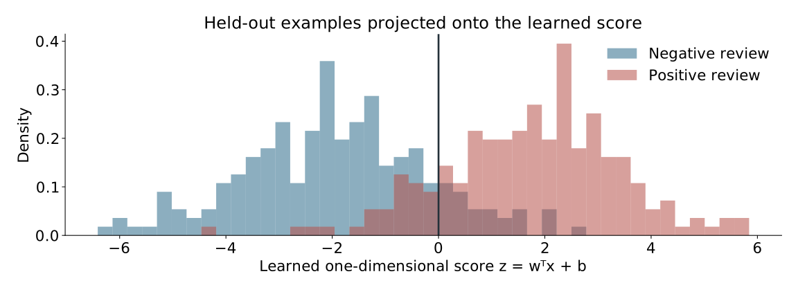
The weights are learned from training reviews; these distributions show held-out reviews.

About two minutes. The displayed x uses training-fitted TF–IDF; w and b were fit only on training examples, with regularization chosen on validation. The test labels color the diagnostic distributions but did not choose the projection or zero threshold. Histograms normalize within each class. A one-dimensional score does not mean all 18,746-dimensional inputs lie on a line.

Next: learn the predictive direction from labels

KNN asks which stored examples are nearby. A linear model learns how much each input contributes to one predictive score.

PCA preserves input variation; our goal is to separate outcomes.

Arc 4: How do labels tell us which weights to learn—and what can a linear score miss?

About one minute. Consolidate the PCA contrast and model-family handoff here. The score/projection visual has already introduced w^T x+b; do not repeat the classifier formula or preview an optimization syllabus. Linear models have not yet been taught. Next arc introduces the objective, fitting, and regularization. PCA/SVD is not a measured baseline for these reviews; do not claim it never helps. A predictive scalar score need not imply a one-dimensional input manifold. This is a different family of predictors f, not merely another value of k. All development/evaluation boundaries still apply to the learned direction.