Learning and Interpreting Linear Regression

David I. Inouye

A new function class changes how we predict

Previously: KNN predicts from nearby stored examples.

Now: learn a shared function that combines the input coordinates.

We begin with house prices, then return to review sentiment.

30 seconds. Arc 3 ended with the motivation for learning a compact predictive score. Do not reteach its empirical comparisons.

First solve a model exactly; then learn how to optimize

Stage	Question
1. Regression → now	Which function, which loss, and what does the OLS solution mean?
2. Classification	How do probabilities change the model and loss?
3. Convexity	What makes these fitting problems well behaved?
4. Optimization	How can local information guide numerical updates?
5. Model limits	What can no linear fit express?

30 seconds. Preserve this roadmap as a hierarchy, not five unrelated methods. Regularization and evaluation recur where needed.

Real Ames sales give us a numerical prediction task

Goal: predict a house’s sale price from its recorded characteristics.

• 2,930 real sales in Ames, Iowa, 2006–2010.
• Inputs include living area, construction year, bathrooms, and neighborhood.
• The target \(y\) is a dollar amount, rather than a class label.

This is regression: predict a numerical outcome.

source:ames-housing-data; source:ames-housing-documentation. Keep historical within-city scope explicit. All records retained; no outlier deletion or target logarithm. This dataset anchors the entire regression segment.

A property becomes a vector of interpretable measurements

Coordinate	Meaning	Example unit
Living area	Above-ground finished space	Square feet
Year built	Construction year	Calendar year
Garage capacity	Number of cars accommodated	Cars
Neighborhood indicator	Membership in one recorded neighborhood	0 or 1

Indicator encoding: turn a category into 0/1 columns.

\[A\mapsto[1,0],\qquad B\mapsto[0,1],\qquad C\mapsto[0,0]\ \text{(reference)}.\]

75 property fields → 226 numerical coordinates after encoding.

source:ames-housing-data; source:ames-housing-documentation. Exclude Order/PID, Sale Type/Condition, Mo Sold/Yr Sold. Numeric medians/scaling and categorical grouping learned only on 1758 training examples. This is hundreds of dimensions, not the review vocabulary scale.

KNN can predict a number by averaging nearby outcomes

For the \(k\) nearest training inputs, indexed by \(N_k(\boldsymbol{x})\):

\[\widehat f_{\mathcal D}(\boldsymbol{x})=\frac1k\sum_{i\in N_k(\boldsymbol{x})}y_i.\]

Three neighboring sales: $150,000, $180,000, and $210,000 → $180,000.

The lookup mechanism is familiar; averaging replaces the classification vote.

The three sale prices are an invented arithmetic example, not three selected Ames records. k is chosen on validation; this procedure did not explicitly minimize a global training objective.

The same sales support a local rule or a single fitted line

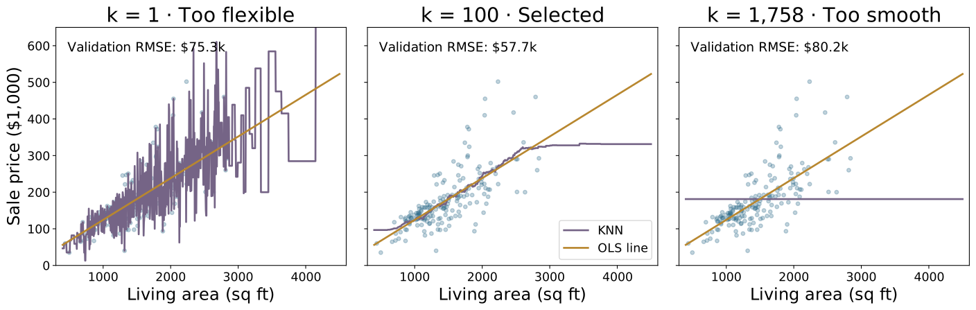
Same training sales and living area alone: small \(k\) follows local fluctuations; very large \(k\) loses the trend.

\(k=100\) is within 0.3% of the best validation RMSE across all \(k\).

source:ames-housing-data. Three panels retain the same 180 displayed training points, identical axes, full 1758-row training set, and OLS line. k=1 exhibits high local sensitivity and poor validation error; k=1758 is the constant training mean and underfits the area trend. k=100 was selected from the original candidate grid; an all-k validation audit finds k=111 with RMSE57549.85 versus57676.68 at100 (0.22% higher). k=1 RMSE75304.58; k=1758 RMSE80158.28. No test outcomes used in this added comparison. These are one-coordinate regressors, not the 226-feature evaluation.

A parametric model learns shared coefficients

KNN regression	Linear regression
Retain examples; find neighbors for each query.	Fit coefficients; reuse the same formula for every query.
The stored model grows with the dataset.	For fixed features, the number of coefficients stays fixed.
Nonparametric	Parametric

These names describe model structure, not whether a method has settings such as \(k\).

Brief contrast only. Nonparametric does not mean assumption-free or devoid of hyperparameters. Our linear fit will use an explicit objective; do not assert every parametric method must be trained this way.

A line predicts with a slope and an offset

\[\widehat y=f_{w,b}(x)=wx+b.\]

• \(x\): measured living area; \(\widehat y\): predicted price.
• \(w\): change in prediction per additional square foot.
• \(b\): where the fitted line meets the vertical axis.

For the one-input Ames fit: 100 more sq ft → about $11,400 more predicted price.

source:ames-housing-data. One-feature training OLS slope is $113.8223/sq ft and intercept $10588.62. It is an association, not a causal effect of renovations. A zero-area house lies outside the useful interpretation of this intercept.

More inputs give a weighted sum of contributions

\[\widehat y=\boldsymbol{w}^{\mathsf T}\boldsymbol{x}+b =\sum_{j=1}^d w_jx_j+b.\]

A coefficient \(w_j\) changes the prediction per unit of \(x_j\), holding the other coordinates fixed.

With 226 input coordinates, there are 227 coefficients including the offset.

The conventional name is “linear model”; the offset makes this formally affine.

Parameters are shared across all observations. Separate measured features, fitted coefficients, and computed predictions. Some combinations of fixed property coordinates are not physically realizable.

Fitted coefficients determine differences in predicted price

Rounded coefficients from the four-feature Ames model:

Feature	Coefficient per unit
Living area (sq ft)	+$90
Construction year	+$840
Full bathrooms	−$11,500
Garage spaces	+$23,600

Compare two houses: same year and bathrooms; house B has 100 more sq ft and one fewer garage space.

\[\widehat y_B-\widehat y_A\approx 100(90)-23{,}600=-\$14{,}600.\]

source:ames-housing-data. Instructor explicitly requests all four coefficients. Coefficients rounded for easy arithmetic; exact area89.9841/year842.3282/bathrooms-11489.9741/garage23614.0284. Exact predicted difference is -14615.62 dollars. Offset cancels, as do the unchanged year and bathroom contributions. This is a comparison of model predictions, not causal effects. Defer overlap/correlated-feature interpretation to the parking lot; do not introduce it here.

Choosing a function leaves which coefficients? unresolved

Established: every \((\boldsymbol{w},b)\) gives a prediction rule.

Next: quantify fitting error, solve for coefficients, and interpret the solution.

Our KNN procedure had no explicit training-objective minimization. Here we will explicitly minimize squared prediction error.

30 seconds. This is the objective transition, not an introduction to iterative optimization.

Residuals measure vertical prediction errors

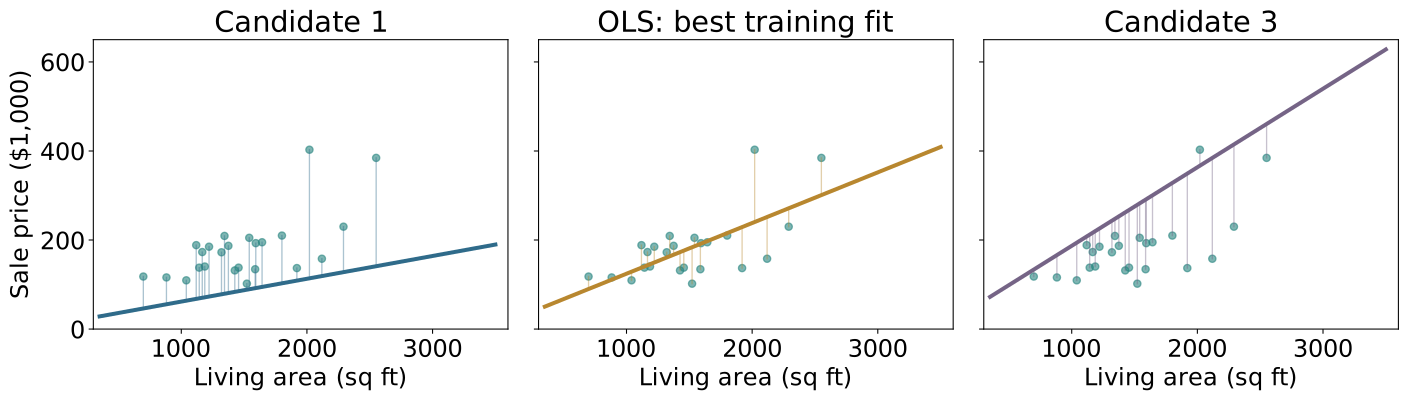
\(r_i=y_i-\widehat y_i\): observed price minus predicted price for house \(i\).

Stack the errors: \(\boldsymbol{r}=[r_1,\ldots,r_n]^{\mathsf T}\in\mathbb{R}^n\) — \(n\) observations, not \(d\) input features.

source:ames-housing-data. Three candidate lines, same 24 displayed sales and axes. Middle gold line is the OLS optimum on all1758training observations. Other slopes are .45 and1.55 times the OLS slope, with the same intercept. Vertical residuals shown for each; do not imply the optimum was fitted only to the24 shown observations.

Mean squared error makes large residuals costly

\[\operatorname{MSE}=\frac1n\sum_{i=1}^n(\widehat y_i-y_i)^2, \qquad J(\boldsymbol{w},b)=\frac12\operatorname{MSE}.\]

Doubling a residual multiplies its squared contribution by four.

The factor \(1/2\) simplifies derivatives; it does not change the minimizer.

For interpretation: \(\operatorname{RMSE}=\sqrt{\operatorname{MSE}}\) is a standard-deviation-like error scale in dollars, rather than dollars squared.

For fitting: minimize squared error; taking the square root adds no new minimizer and complicates the derivatives.

Squared loss is a modeling choice, not a defining requirement of regression. RMSE is not mean absolute error. It equals the residual standard deviation with divisor n when residual mean is zero (as for training OLS with an intercept); otherwise its square includes squared mean error. RMSE could be optimized and has the same minimizers by monotonicity, but use MSE for simpler algebra and smoothness at zero residual. No degrees-of-freedom correction is being taught. Squared loss is sensitive to unusual large errors.

Can large positive and negative errors cancel the fitting problem?

A model makes two residuals: +$50,000 and −$50,000.

What does their zero average establish?

A. The model has zero mean squared error.

B. The signs balance, but squared error can still be large.

C. The fitted line must be the least-squares solution.

B. Squaring prevents opposite signs from hiding large mistakes.

Two-minute check. Zero average residual alone does not imply optimal slope, good predictions, or generalization.

First solve one input and one fitted line

Simplify to build intuition: living area \(x\) predicts price \(y\) using \(wx+b\).

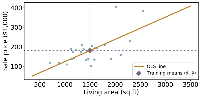
At \(x=\bar x\), choosing \(b=\bar y-w\bar x\) gives \(w\bar x+b=w\bar x+(\bar y-w\bar x)=\bar y\).

This places the line through \((\bar x,\bar y)\). Why is that offset optimal?

source:ames-housing-data. Preview the fitted line and its full-training mean before the derivative. For any fixed slope this offset puts the line through the means; that alone does not determine the best slope. Next derive the optimal offset, then the slope.

Optimizing the offset balances the residuals

\(J(w,b)=\frac1{2n}\sum_i(wx_i+b-y_i)^2\).

\(\displaystyle \frac{\partial J}{\partial b}\)

\(=\)

\(\displaystyle \frac1n\sum_i(wx_i+b-y_i)\)

(Differentiate each squared residual)

\(\displaystyle \,\)

\(=\)

\(\displaystyle w\frac1n\sum_i x_i+b-\frac1n\sum_i y_i\)

(Distribute the sum; b repeats n times)

\(\displaystyle 0\)

\(=\)

\(\displaystyle w\bar x+b-\bar y\)

(Set the derivative to zero)

\(\displaystyle \widehat b(w)\)

\(=\)

\(\displaystyle \bar y-w\bar x\)

(Solve for b at a fixed slope)

The intercept derivative is the mean prediction error: this choice makes it zero.

For fixed w, the second derivative with respect to b is1, so this stationary offset is the unique minimum. Note b-hat(w) depends on the slope; the final offset uses w-hat.

Substituting the offset centers both inputs and outcomes

Write \(x_i^c=x_i-\bar x\) and \(y_i^c=y_i-\bar y\).

\(\displaystyle wx_i+\widehat b(w)-y_i\)

\(=\)

\(\displaystyle wx_i+(\bar y-w\bar x)-y_i\)

(Substitute the optimal offset)

\(\displaystyle \,\)

\(=\)

\(\displaystyle w(x_i-\bar x)-(y_i-\bar y)=wx_i^c-y_i^c\)

(Collect centered quantities)

\(\displaystyle \frac{d}{dw}J(w,\widehat b(w))\)

\(=\)

\(\displaystyle \frac1n\sum_i x_i^c(wx_i^c-y_i^c)\)

(Differentiate the centered squared errors)

Now set this derivative to zero and solve for the slope.

The reduced objective is J(w,bhat(w))=(1/2n)sum(wxci-yci)^2. Centered values are fixed training data, not functions of w.

Rearranging the zero derivative gives the closed-form slope

\(\displaystyle 0\)

\(=\)

\(\displaystyle \sum_i x_i^c(\widehat w x_i^c-y_i^c)\)

(Set derivative to zero; multiply by n)

\(\displaystyle \,\)

\(=\)

\(\displaystyle \sum_i\left[\widehat w(x_i^c)^2-x_i^cy_i^c\right]\)

(Distribute each product)

\(\displaystyle \,\)

\(=\)

\(\displaystyle \widehat w\sum_i(x_i^c)^2-\sum_i x_i^cy_i^c\)

(Take the shared slope outside the sum)

\(\displaystyle \widehat w\sum_i(x_i^c)^2\)

\(=\)

\(\displaystyle \sum_i x_i^cy_i^c\)

(Move the cross-products to the other side)

\(\displaystyle \widehat w\)

\(=\)

\(\displaystyle \frac{\sum_i x_i^cy_i^c}{\sum_i(x_i^c)^2}\)

(Divide by the input sum of squares)

Assume nonconstant x, so denominator positive. Then bhat=ybar-what*xbar. The factor1/n cancels; ratio of the corresponding averages is identical.

Each observation contributes a signed product and a squared distance

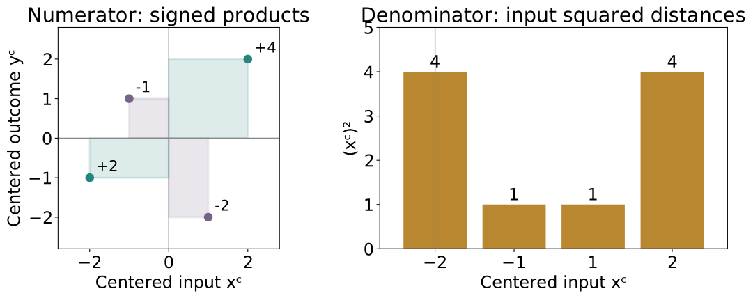
Toy centered data: numerator \(=2-1-2+4=3\); denominator \(=4+1+1+4=10\).

Same-sign deviations support a positive slope; opposite signs oppose it. Here \(\widehat w=3/10\).

Explicit toy example, not Ames values. x-centered=[-2,-1,1,2], y-centered=[-1,1,-2,2], both sum0. Rectangle area magnitudes equal absolute cross-products; colors encode signs. Right bars show squared input deviations. Geometry explains individual terms, not just the final ratio.

The fitted slope is a weighted average of slopes from the mean

For observations with \(x_i^c\ne0\):

\[\widehat w=\sum_i\underbrace{\frac{(x_i^c)^2}{\sum_j(x_j^c)^2}}_{\text{weight, summing to 1}} \underbrace{\frac{y_i^c}{x_i^c}}_{\text{slope from the mean point}}.\]

Inputs farther from the mean have more weight in determining the slope.

Dividing by \(\sum_i(x_i^c)^2\) normalizes the weights. It is not an unweighted average of the individual slopes.

Finally, \(\widehat b=\bar y-\widehat w\bar x\) positions this slope through the mean point.

Terms with xci=0 contribute zero to numerator and denominator and are excluded from the slope-ratio expression; do not evaluate0/0. Units are dollars/sqft for Ames. This is an algebraic interpretation of the existing solution, not a new estimation method.

Stacking predictions turns the problem into one matrix equation

Put observations in rows of \(X\in\mathbb R^{n\times d}\).

\[\widetilde X=[X\;\boldsymbol{1}],\qquad \boldsymbol{\theta}=\begin{bmatrix}\boldsymbol{w}\\b\end{bmatrix}, \qquad \widehat{\boldsymbol{y}}=\widetilde X\boldsymbol{\theta}.\]

\[J(\boldsymbol{\theta})=\frac1{2n}\|\widetilde X\boldsymbol{\theta}-\boldsymbol{y}\|_2^2.\]

Shape check: \((n\times(d+1))((d+1)\times1)=n\times1\) predictions.

The observed outcomes, predictions, and residuals are n-vectors: one entry per observation. Each individual input is instead a d-vector: one entry per feature. Realized response vector y is bold italic. The final column of ones accounts for the offset. Reuse Arc 2 shapes; the observation columns remain column vectors in single-example formulas.

Write squared error as an inner product before expanding

\(\displaystyle J(\boldsymbol{\theta})\)

\(=\)

\(\displaystyle \frac1{2n}\|\widetilde X\boldsymbol{\theta}-\boldsymbol{y}\|_2^2\)

(Squared-residual form)

\(\displaystyle \,\)

\(=\)

\(\displaystyle \frac1{2n}(\widetilde X\boldsymbol{\theta}-\boldsymbol{y})^{\mathsf T}(\widetilde X\boldsymbol{\theta}-\boldsymbol{y})\)

(A squared norm is an inner product)

\(\displaystyle \,\)

\(=\)

\(\displaystyle \frac1{2n}(\boldsymbol{\theta}^{\mathsf T}\widetilde X^{\mathsf T}-\boldsymbol{y}^{\mathsf T})(\widetilde X\boldsymbol{\theta}-\boldsymbol{y})\)

(Transpose the difference)

Recall transpose reverses product order. All dimensions match: residuals are n-vectors and the inner product is scalar.

The expansion contains two equal scalar cross terms

\(\displaystyle 2nJ(\boldsymbol{\theta})\)

\(=\)

\(\displaystyle \begin{aligned}[t]&\boldsymbol{\theta}^{\mathsf T}\widetilde X^{\mathsf T}\widetilde X\boldsymbol{\theta}-\boldsymbol{\theta}^{\mathsf T}\widetilde X^{\mathsf T}\boldsymbol{y}\\&{}-\boldsymbol{y}^{\mathsf T}\widetilde X\boldsymbol{\theta}+\boldsymbol{y}^{\mathsf T}\boldsymbol{y}\end{aligned}\)

(Multiply out all four terms)

\(\displaystyle \boldsymbol{y}^{\mathsf T}\widetilde X\boldsymbol{\theta}\)

\(=\)

\(\displaystyle (\boldsymbol{y}^{\mathsf T}\widetilde X\boldsymbol{\theta})^{\mathsf T}=\boldsymbol{\theta}^{\mathsf T}\widetilde X^{\mathsf T}\boldsymbol{y}\)

(A scalar equals its transpose)

\(\displaystyle 2nJ(\boldsymbol{\theta})\)

\(=\)

\(\displaystyle \boldsymbol{\theta}^{\mathsf T}\widetilde X^{\mathsf T}\widetilde X\boldsymbol{\theta}-2\boldsymbol{\theta}^{\mathsf T}\widetilde X^{\mathsf T}\boldsymbol{y}+\boldsymbol{y}^{\mathsf T}\boldsymbol{y}\)

(Combine the cross terms)

Use full width for this expansion. Scalar transpose equality is the essential bridge, not symmetry of an arbitrary matrix.

Differentiate each term, then set the gradient to zero

The matrix \(\widetilde X^{\mathsf T}\widetilde X\) is symmetric.

Term in \(2nJ\)	Gradient with respect to \(\boldsymbol{\theta}\)
\(\boldsymbol{\theta}^{\mathsf T}\widetilde X^{\mathsf T}\widetilde X\boldsymbol{\theta}\)	\(2\widetilde X^{\mathsf T}\widetilde X\boldsymbol{\theta}\)
\(-2\boldsymbol{\theta}^{\mathsf T}\widetilde X^{\mathsf T}\boldsymbol{y}\)	\(-2\widetilde X^{\mathsf T}\boldsymbol{y}\)
\(\boldsymbol{y}^{\mathsf T}\boldsymbol{y}\)	\(\boldsymbol{0}\): independent of the coefficients

\(\displaystyle \nabla J(\boldsymbol{\theta})\)

\(=\)

\(\displaystyle \frac1{2n}(2\widetilde X^{\mathsf T}\widetilde X\boldsymbol{\theta}-2\widetilde X^{\mathsf T}\boldsymbol{y}+\boldsymbol{0})\)

(Combine the term derivatives)

\(\displaystyle \,\)

\(=\)

\(\displaystyle \frac1n(\widetilde X^{\mathsf T}\widetilde X\boldsymbol{\theta}-\widetilde X^{\mathsf T}\boldsymbol{y})\)

(Cancel the factor of two)

\(\displaystyle \boldsymbol{0}\)

\(=\)

\(\displaystyle \frac1n(\widetilde X^{\mathsf T}\widetilde X\widehat{\boldsymbol{\theta}}-\widetilde X^{\mathsf T}\boldsymbol{y})\)

(Set the gradient to zero)

\(\displaystyle \widetilde X^{\mathsf T}\widetilde X\widehat{\boldsymbol{\theta}}\)

\(=\)

\(\displaystyle \widetilde X^{\mathsf T}\boldsymbol{y}\)

(Multiply by n; rearrange)

The quadratic derivative differentiates both coefficient factors. The two contributions agree because Xtilde-transpose Xtilde is symmetric. This is solving stationarity equations, not gradient descent.

Independent columns give the OLS inverse formula

If \(\widetilde X\) has full column rank:

\[\boxed{\widehat{\boldsymbol{\theta}}= (\widetilde X^{\mathsf T}\widetilde X)^{-1}\widetilde X^{\mathsf T}\boldsymbol{y}.}\]

• \(\widetilde X^{\mathsf T}\boldsymbol{y}\) measures feature–outcome alignment.
• \(\widetilde X^{\mathsf T}\widetilde X\) records feature sizes and overlap.
• Its inverse accounts for that overlap when assigning coefficients.

In code, use a least-squares solver, rather than explicitly forming the inverse.

Full column rank implies invertible Gram matrix. QR/SVD compute the solution more reliably than explicitly forming the inverse. Correlation between columns means coefficients are not independent marginal correlations.

At the solution, residuals are orthogonal to every feature column

Let \(\boldsymbol{r}=\boldsymbol{y}-\widetilde X\widehat{\boldsymbol{\theta}}\in\mathbb{R}^n\): one residual per observation, not per feature.

Each column of \(\widetilde X\in\mathbb{R}^{n\times(d+1)}\) also has \(n\) entries: one feature measured across all observations.

\(\displaystyle \widetilde X^{\mathsf T}\boldsymbol{r}\)

\(=\)

\(\displaystyle \widetilde X^{\mathsf T}(\boldsymbol{y}-\widetilde X\widehat{\boldsymbol{\theta}})\)

(Substitute the residual vector)

\(\displaystyle \,\)

\(=\)

\(\displaystyle \widetilde X^{\mathsf T}\boldsymbol{y}-\widetilde X^{\mathsf T}\widetilde X\widehat{\boldsymbol{\theta}}\)

(Distribute the matrix product)

\(\displaystyle \,\)

\(=\)

\(\displaystyle \boldsymbol{0}\)

(Use the normal equations)

Each feature column has zero dot product with the residual vector: no residual component lies along a direction the model can adjust.

The column of ones also gives \(\sum_i r_i=0\): overpredictions and underpredictions balance.

Use the normal equations directly. This is training-sample orthogonality, not probabilistic independence or a statement about unseen errors. Two minutes including interpretation. The residual is perpendicular to every attainable change in the fitted response vector.

OLS projects the outcome vector onto possible fitted vectors

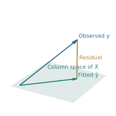
The plane represents \(\operatorname{col}(\widetilde X)\); the residual is perpendicular to it.

Illustrative three-dimensional response-space geometry, not a plot of living area versus price. Axes represent coordinates of stacked outcomes after a rotation. In Ames this response space has n=1758 dimensions. The model predictions lie in a subspace; this is a different space from the earlier input scatterplot.

Orthogonality proves that no other fit has lower error

• \(\boldsymbol{r}=[r_1,\ldots,r_n]^{\mathsf T}\in\mathbb{R}^n\): one residual per observation, \(r_i=y_i-\widehat y_i\).
• \(\boldsymbol{r}\) has \(n\) coordinates for observations, not \(d\) coordinates for features like \(\boldsymbol{x}_i\).
• Recall OLS orthogonality: \(\widetilde X^{\mathsf T}\boldsymbol{r}=\boldsymbol{0}\); \(\boldsymbol{r}\) is perpendicular to each \(n\)-dimensional feature column.

Any other coefficient vector is \(\widehat{\boldsymbol{\theta}}+\boldsymbol{\delta}\); its prediction change \(\widetilde X\boldsymbol{\delta}\in\mathbb{R}^n\).

\(\displaystyle \|\boldsymbol{y}-\widetilde X(\widehat{\boldsymbol{\theta}}+\boldsymbol{\delta})\|^2\)

\(=\)

\(\displaystyle \|\boldsymbol{r}-\widetilde X\boldsymbol{\delta}\|^2\)

(Write the new residual)

\(\displaystyle \,\)

\(=\)

\(\displaystyle \|\boldsymbol{r}\|^2+\|\widetilde X\boldsymbol{\delta}\|^2\)

(\(\boldsymbol{r}^{\mathsf T}(\widetilde X\boldsymbol{\delta})=0\))

\(\displaystyle \,\)

\(\ge\)

\(\displaystyle \|\boldsymbol{r}\|^2\)

(A squared norm is nonnegative)

The bound is attained: choose \(\boldsymbol{\delta}=\boldsymbol{0}\), so \(\|\widetilde X\boldsymbol{\delta}\|^2=0\).

Thus \(\widehat{\boldsymbol{\theta}}\) achieves the smallest possible squared error, \(\|\boldsymbol{r}\|^2\): it is a global minimum.

Before the algebra, distinguish the spaces: n indexes observations (houses), d indexes features of one house. Both the stacked predictions and residuals have n coordinates. A feature column of the design matrix also has n coordinates, so its orthogonality with residuals is a dot product across observations, not across features. Here n=1758 training houses and d=226 encoded inputs; theta and delta have d+1 coordinates including the intercept. Zero delta is always optimal; it is the only optimal delta when the design has independent columns. Otherwise any delta in the null space also attains the bound, anticipating the redundancy slide. The omitted cross term is -2 r^T Xtilde delta = -2 (Xtilde^T r)^T delta=0. Reveal that justification with the second equality, not later. This establishes global optimality without assuming convexity already taught.

Does zero training residual alignment imply perfect prediction?

The OLS solution satisfies \(\widetilde X^{\mathsf T}\boldsymbol{r}=\boldsymbol{0}\).

Which conclusion follows?

A. Every residual is zero.

B. No linear coefficient adjustment reduces the training squared error.

C. The model will have zero error on future houses.

B. A nonzero residual can be perpendicular to the entire prediction subspace.

Two minutes. Transfer the projection geometry to distinguish optimality from interpolation and generalization. A vector can be nonzero yet orthogonal to every feature column. No test-data inference follows from the normal equations.

Redundant features can give the same fit with different coefficients

Example: predict a venue’s booking price from its room capacities (zero offset).

Feature	Seats	Model A coefficient	Model B coefficient
Room 1: \(x_1\)	20	1	0
Room 2: \(x_2\)	30	2	1
Total: \(x_3=x_1+x_2\)	50	0	1

\[\widehat y_A=1(20)+2(30)+0(50)=80,\qquad \widehat y_B=0(20)+1(30)+1(50)=80.\]

Same for every venue: \(x_2+x_3=x_1+2x_2\) whenever \(x_3=x_1+x_2\).

The data cannot distinguish these coefficient choices.

The inverse formula requires independent columns; redundant columns make \(\widetilde X^{\mathsf T}\widetilde X\) singular.

The room capacities, coefficients (dollars per seat), and booking prices are invented for arithmetic; no empirical booking-price claim. Both models use zero offset. Their weight difference is (-1,-1,1), whose dot product with every valid input is zero because total capacity is the sum of the two rooms. This is exact structural redundancy, not merely high correlation or a coincidence for the 20/30 example. Least squares still has a solution: remove redundancy or use an SVD-based solver. Individual coefficients need care; predictions are uniquely determined on the represented subspace. source:ames-housing-data. Full encoded Ames training matrix has centered rank219 versus226 features. The numerical comparison uses SVD least squares, not an invalid inverse. Fitted training responses are unique; test responses can differ for dependencies that do not persist. Do not turn this into a long numerical-analysis detour.

On real Ames sales, ordinary least squares is competitive

Same split: 1,758 train / 586 validation / 586 test; 226 encoded coordinates.

Model	Test RMSE ↓
Predict the training mean	$78,500
Validation-selected KNN	$32,800
Ordinary least squares	$26,300
Random forest	$25,700
Boosted trees	$25,200

A compact linear rule is useful here even alongside flexible nonlinear methods.

source:ames-housing-data; source:ames-housing-documentation. Fixed seed570, no test selection or outlier removal, train-only preprocessing. Tree methods are empirical reference points, not new methods taught here. One split supports competitiveness here, not universal superiority. RMSE is not a typical absolute-error guarantee; OLS MAE16400.

Held-out predictions reveal both useful structure and remaining errors

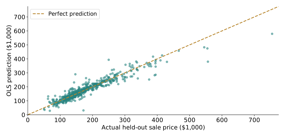
Each dot is one of 586 test sales. The diagonal means prediction equals outcome.

source:ames-housing-data. Full 226-coordinate OLS model, same fixed test split as the table. This is neither the one-input line nor training-fit evidence. Large expensive-house misses remain; aggregate error does not guarantee uniform accuracy across prices. Scope is historical Ames sales with this representation and split.

Solving the training problem leaves the prediction claim to evaluate

We can now explain: the function, the squared-error objective, the exact solution, and its geometry.

An exact fit to the objective does not make the model exact about the world.

Next: keep the linear score, but change from house prices to class probabilities.

30 seconds. Natural first-meeting boundary. Preserve train/validation/test as an established principle without repeating its full derivation.