From Linear Scores to Class Probabilities

David I. Inouye

Classification changes what the score must predict

Regression: a numerical price, \(\widehat y=\boldsymbol{w}^{\mathsf T}\boldsymbol{x}+b\).

Classification: a positive/negative review, with an estimated class probability.

Return to our real Cornell case: 18,746 word features, 1,200 training reviews.

source:cornell-movie-review-polarity-v2; source:cornell-movie-review-polarity-v2-data. Thirty-second orientation; the case was motivated in Arc3.

Logistic regression follows model → objective → solution

1. Model — now: turn the score into a probability.

2. Objective — next: measure how well those probabilities predict the labels.

3. Solution — afterward: learn the coefficients by numerical optimization.

Thirty-second section divider after motivating the return to classification. Orient students to the same model–objective–solution progression used for linear regression; optimization is developed later.

A learned score combines signed contributions

For one review, let \(\boldsymbol{x}\in\mathbb R^d\) contain its word features.

\[ z=\boldsymbol{w}^{\mathsf T}\boldsymbol{x}+b =\sum_{j=1}^d w_jx_j+b. \]

• \(x_j\): the review’s measured feature; given at prediction time.
• \(w_j\): how that feature contributes; learned from labeled reviews.
• \(b\): a learned offset; \(z\): the resulting scalar score.

With \(d=18{,}746\), the model learns 18,747 parameters, not one parameter per review.

Three minutes. The corpus and feature count are from source:cornell-movie-review-polarity-v2 and source:cornell-movie-review-polarity-v2-data. Do not teach TF–IDF here. Distinguish observed x, learned w and b, and computed z. A scalar output need not imply that the input distribution lies on a line. Formally this score is affine when b is nonzero; “linear model” is the usual family name. Parameters are shared across all examples.

Each contribution is a weight times a measurement

Illustrative two-feature review, with invented weights:

Feature	Measurement \(x_j\)	Weight \(w_j\)	Contribution \(w_jx_j\)
“engaging”	2	\(+0.8\)	\(+1.6\)
“dull”	1	\(-1.1\)	\(-1.1\)
Offset	—	\(b=-0.2\)	\(-0.2\)

\[z=1.6-1.1-0.2=0.3\quad\Longrightarrow\quad\widehat y=1.\]

The model combines evidence; a word’s contribution depends on both its value and its weight.

Two minutes. These are invented counts and coefficients for arithmetic, not estimated coefficients from the review experiment. Use the zero threshold previewed last time; the next slide gives its geometry. Positive is label 1. The additive word representation does not model negation or word order.

A zero threshold divides space with a hyperplane

\[ \widehat y=\mathbf1\{\boldsymbol{w}^{\mathsf T}\boldsymbol{x}+b\ge0\}, \qquad \text{boundary: }\boldsymbol{w}^{\mathsf T}\boldsymbol{x}+b=0. \]

• In two dimensions, the boundary is a line; in three, a plane.
• \(\boldsymbol{w}\) determines its orientation; \(b\) shifts its position.
• Moving in a direction orthogonal to \(\boldsymbol{w}\) leaves the score unchanged.

Learning chooses which direction matters for the labels, rather than which examples are nearby in every coordinate.

Three minutes. Draw a two-dimensional line and its normal. For w nonzero, adding v with w^T v=0 preserves z. The score is a scaled projection plus an offset, not necessarily an orthogonal coordinate because w need not be a unit vector. PCA chose a direction for input variation; our objective will use outcomes.

A sigmoid converts the score into a probability estimate

\[ \widehat\eta(\boldsymbol{x})=\sigma(z)=\frac{1}{1+e^{-z}}, \qquad z=\boldsymbol{w}^{\mathsf T}\boldsymbol{x}+b. \]

Score \(z\)	Probability of label 1
\(-4\)	1.8%
\(-2\)	11.9%
\(0\)	50%
\(2\)	88.1%
\(4\)	98.2%

Logistic regression uses this probability model.

Three minutes. The analytic S curve marks the five table values and the zero-score/half-probability midpoint. It approaches but never reaches zero or one at a finite score. Figure regenerated with lectures/scripts/arc4_sigmoid.py. Eta-hat estimates Pr(y=1 given x); it is not the unknown population eta itself. Despite its name, logistic regression is commonly used for classification. Sigmoid is strictly increasing, so its one-half threshold preserves the zero-score boundary.

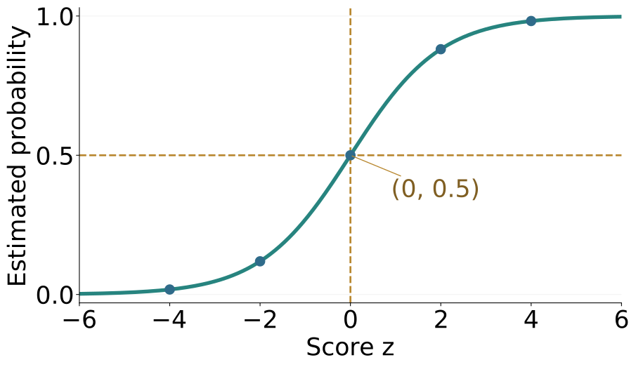
The probability changes smoothly; the class boundary stays linear

\[ \widehat\eta(\boldsymbol{x})\ge\tfrac12 \quad\Longleftrightarrow\quad \boldsymbol{w}^{\mathsf T}\boldsymbol{x}+b\ge0. \]

• A larger positive score means a larger estimated probability of label 1.
• Multiplying all coefficients by 10 keeps the decisions but makes probabilities more extreme.
• An S-shaped probability function does not make this decision boundary curved.

Two minutes. Connect to the sigmoid and its one-half threshold. Confidence and classification are different outputs. For a fixed threshold other than one-half, the boundary is still a hyperplane with a different offset. Do not introduce threshold tuning as another activity here.

The probability model is fixed; now choose the fitting objective

Model: a linear score followed by a sigmoid.

Now: what loss should tell us whether its probabilities fit the labels?

Next: solve for the coefficients that minimize that loss.

30 seconds. Return to the model → objective → solution roadmap. The previous slides defined the output and decision boundary. Accuracy’s flat regions now motivate a smooth probability-fitting objective; log loss is a modeling choice, not an automatic consequence of the sigmoid.

Accuracy gives little guidance between boundary crossings

For one positive review, compare scores \(z=-3\) and \(z=-0.1\).

Score	Predicted probability	Predicted class	Classification error
\(-3\)	4.7%	0	1
\(-0.1\)	47.5%	0	1

The probability moved toward the observed label, but accuracy sees no improvement yet.

A smooth loss can provide information about such changes before the class flips.

Three minutes. Accuracy remains an evaluation criterion. Its stepwise training objective is locally flat almost everywhere, so ordinary gradient updates receive no useful local signal. We are choosing a useful surrogate, not claiming accuracy is an invalid goal or that its optimization is impossible by every method.

Log loss rewards probability assigned to the observed outcome

Let \(a=\widehat\eta(\boldsymbol{x})\) and \(y\in\{0,1\}\).

\[ \ell(y,a)=-y\log a-(1-y)\log(1-a) =\begin{cases}-\log a,&y=1,\\-\log(1-a),&y=0.\end{cases} \]

Give the observed outcome high probability → small loss.

Give the observed outcome nearly zero probability → large loss.

Three minutes. Natural logarithms; a is strictly between zero and one for finite logistic scores. This is binary cross-entropy or negative log likelihood for one Bernoulli observation. Introduce the meaning before deriving the full objective.

Confident mistakes receive a larger penalty

For a positive outcome, \(y=1\):

Predicted probability \(a\)	Class at threshold 0.5	Log loss \(-\log a\)
0.99	Correct	0.010
0.60	Correct	0.511
0.40	Wrong	0.916
0.01	Wrong	4.605

Unlike classification error, log loss distinguishes how confidently a prediction was made.

Two minutes. Have students compare the two wrong predictions and the two correct ones. A single confidently wrong observation can matter greatly; the objective is not simply a count of wrong classifications.

Would accuracy and log loss choose the same model?

Two observed outcomes are both positive: \(y_1=y_2=1\).

Model	Predicted probabilities	Accuracy	Average log loss
A	\((0.60,\;0.60)\)	100%	0.511
B	\((0.99,\;0.49)\)	50%	0.362

What does this comparison establish?

A. Accuracy and log loss always rank models identically.

B. Better log loss can coexist with worse thresholded accuracy.

C. Model B must generalize better to every new population.

B. The criteria assess different outputs. Neither two-example score establishes population performance.

Two minutes. Let students choose, then explain that smooth probability fitting is a surrogate, not an identical numerical version of classification accuracy. Values use natural logs and threshold one-half. Keep the setup short; no calculator task is required because the losses are supplied.

MSE and log loss express different prediction criteria

Numerical regression	Logistic probability prediction
Output: \(\widehat y=z\)	Output: \(a=\sigma(z)\)
Loss: \(\tfrac12(z-y)^2\)	Loss: \(-y\log a-(1-y)\log(1-a)\)
Penalize numerical residual size.	Penalize low probability of the observed label.

Squared error on probabilities is also possible, but composing it with a sigmoid generally loses convexity in the coefficients.

Do not claim squared error is invalid for classification. Brier loss is convex in probability but not generally in logistic coefficients. Convexity will be defined next; here it motivates the question.

The logistic objective has no general closed-form coefficient solution

With \(z_i=\boldsymbol{w}^{\mathsf T}\boldsymbol{x}_i+b\) and \(a_i=\sigma(z_i)=e^{z_i}/(1+e^{z_i})\):

\[\log a_i=z_i-\log(1+e^{z_i}),\qquad \log(1-a_i)=-\log(1+e^{z_i}).\]

\(\displaystyle \ell(y_i,a_i)\)

\(=\)

\(\displaystyle -y_i\log a_i-(1-y_i)\log(1-a_i)\)

(Usual binary log loss)

\(\displaystyle \,\)

\(=\)

\(\displaystyle -y_i z_i+\big[y_i+(1-y_i)\big]\log(1+e^{z_i})\)

(Substitute the two log identities)

\(\displaystyle \,\)

\(=\)

\(\displaystyle \log(1+e^{z_i})-y_i z_i\)

(Combine the coefficients)

Average the same loss over observations:

\[J(\boldsymbol{w},b)=\frac1n\sum_{i=1}^n\ell(y_i,a_i) =\frac1n\sum_{i=1}^n\left[\log(1+e^{z_i})-y_i z_i\right].\]

OLS gave linear stationary equations; logistic loss gives nonlinear equations in the coefficients.

Next: what does the objective’s shape guarantee?

About three minutes before calibration. Start from the ordinary probability-based binary log loss, not an unexplained score formula. Rewrite sigmoid(z)=exp(z)/(1+exp(z)); its complement is 1/(1+exp(z)). Taking logs gives the two displayed identities. Substitution produces -y z + y log(1+exp(z)) + (1-y) log(1+exp(z)); the logarithm coefficients sum to one. Then average over n observations. This is an exact algebraic re-expression, not a new loss or approximation. Natural logs. Finite z gives 0<a<1. There is no general analytic coefficient formula analogous to OLS, though special cases exist. Next is convexity, not immediately gradient descent.