Why the Shape of the Objective Matters

David I. Inouye

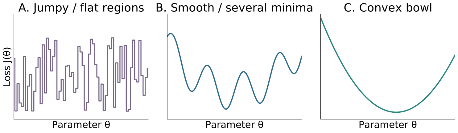
Which loss would be easiest to optimize?

Which shape gives us the clearest route to a global minimum?

A. The jumpy loss.

B. The smooth loss with several minima.

C. The convex bowl.

C. A local minimum is already global; there are no worse local minima to escape.

Two minutes, including the reveal. These are invented one-parameter objectives, not measured model losses. A is a seeded step function: derivatives are zero on flat intervals and undefined at jumps, so a local gradient is not useful. B is a quadratic plus sinusoid with several local minima: smoothness alone does not rule out worse local minima. C is a quadratic. The picture motivates a structural guarantee; it is not a universal runtime comparison.

A useful objective lets us reason about the solution

• Jumpy: a small change may reveal little—or abruptly change the loss.
• Smooth, several minima: downhill progress can end at a worse local minimum.
• Convex: a local minimum is global, making optimality easier to analyze.

Convexity is a useful class of well-behaved objectives.

It gives a global guarantee; speed still depends on the problem and algorithm.

About one minute. An arbitrary objective can hide a better value far from the current point. Without additional structure, local information cannot certify global optimality. Convexity supplies that structure. Do not equate smoothness with convexity or promise that every convex problem is easy to compute. Convex functions can be nonsmooth and can fail to attain a minimum. source:boyd-vandenberghe-convex-optimization.

Objective shape answers three linked questions

1. Define: what does convexity mean geometrically?
2. Check: are our OLS and logistic objectives convex?
3. Interpret: what does that guarantee—and what else do we need?

30 seconds. Connect the next two proofs: the secant inequality defines convexity, and the curvature test gives a practical way to verify it. Then apply the test to our objectives and separate global optimality from uniqueness, existence, and speed.

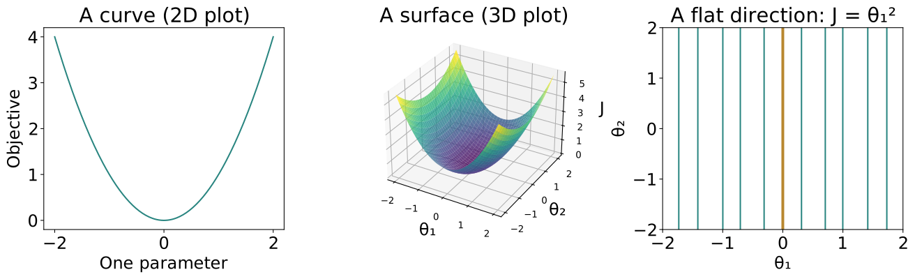
Convexity is a statement about the entire objective shape

A convex objective may have a single bottom—or a flat set of equally good solutions.

source:boyd-vandenberghe-convex-optimization. Geometric views of the same definition: Left: one parameter, 2D plot. Center: two parameters and height,3D plot. Right: contour view of a flat direction. These are mathematical illustrations, not empirical loss fits.

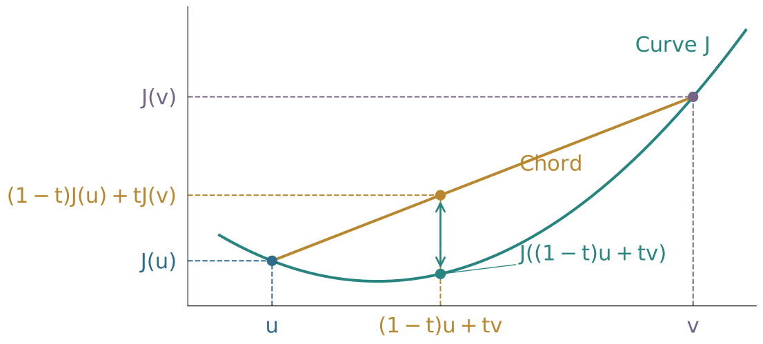
Definition: a convex function lies below every chord

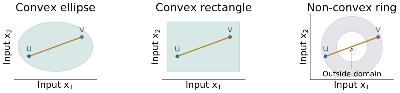
\(J\) is convex on a convex domain if, for every \(\boldsymbol{u},\boldsymbol{v}\) in the domain and \(0\le t\le1\),

\[{\color{#27847f}{J\big(}}{\color{#b8872f}{(1-t)}}{\color{#2f6b8a}{\boldsymbol{u}}}+{\color{#b8872f}{t}}{\color{#756486}{\boldsymbol{v}}}{\color{#27847f}{\big)}} \le {\color{#b8872f}{(1-t)}}{\color{#2f6b8a}{J(\boldsymbol{u})}}+{\color{#b8872f}{t}}{\color{#756486}{J(\boldsymbol{v})}}.\]

Loss at the averaged input ≤ average of the endpoint losses.

source:boyd-vandenberghe-convex-optimization,section3.1.1. Definition, not a claim derived from one drawing. A convex domain contains every weighted average (1-t)u+tv of its points. Plot is the scalar case; bold vectors in the inequality allow multiple coefficients. Blue matches u and J(u), purple matches v and J(v), gold matches both convex combinations. At the same averaged input, the teal curve point is below the gold chord point. The two averages have the same weights but are generally different output values. Point to each labeled axis value before reading the inequality.

Convexity makes every local minimum global

Suppose \(\boldsymbol{u}\) is a local minimum, but some \(\boldsymbol{v}\) has lower loss.

\[J((1-t)\boldsymbol{u}+t\boldsymbol{v})\le(1-t)J(\boldsymbol{u})+tJ(\boldsymbol{v}).\]

Since \(J(\boldsymbol{v})<J(\boldsymbol{u})\), the right side is less than \(J(\boldsymbol{u})\) for every \(t>0\).

Choosing an arbitrarily small \(t\) gives a nearby point with lower loss—a contradiction.

Therefore, a local minimum must be global.

source:boyd-vandenberghe-convex-optimization,section4.2.2. Separate the definition from its first consequence. As t approaches zero the segment point approaches u, remaining in the convex domain. The strict improvement contradicts local minimality.

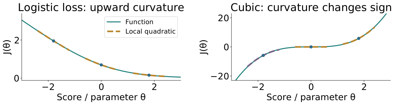
For a twice differentiable function, convexity means nonnegative curvature

Let \(J\) be twice continuously differentiable on an open convex domain.

Parameters	Equivalent criterion for convexity
One scalar \(\theta\)	\(J''(\theta)\ge0\) everywhere
A vector \(\boldsymbol{\theta}\)	\(H(\boldsymbol{\theta})=\nabla^2J(\boldsymbol{\theta})\succeq0\) everywhere

The Hessian is the matrix of second partial derivatives: \(H_{jk}=\frac{\partial^2J}{\partial\theta_j\partial\theta_k}\).

Positive semidefinite (PSD) means \(\boldsymbol{v}^{\mathsf T}H\boldsymbol{v}\ge0\) for every direction \(\boldsymbol{v}\). Equivalently, all eigenvalues of \(H\) are \(\ge0\): no eigenvector direction curves downward; zero allows a flat direction at that point.

Derivation hints: in one dimension, \(J''\ge0\) makes slopes nondecreasing, giving the chord inequality. In several dimensions, restrict to a line:

\[g(t)=J(\boldsymbol{\theta}+t\boldsymbol{v}),\qquad g''(t)=\boldsymbol{v}^{\mathsf T}H(\boldsymbol{\theta}+t\boldsymbol{v})\boldsymbol{v}.\]

source:boyd-vandenberghe-convex-optimization,section3.1.4. State the equivalence instead of deriving it. C2 implies the real Hessian is symmetric, so it has orthogonal eigenvector directions and real eigenvalues. The directional quadratic form weights squared coordinates by eigenvalues; nonnegative eigenvalues are exactly PSD. Require this at every point, not merely at the candidate minimum. Zero eigenvalue means zero second-order curvature there, not necessarily a globally flat function (theta^4 at zero). Interested students: compare mean-value slopes on either side of a point to obtain the secant inequality; in the reverse direction use the midpoint inequality and take a second-difference limit. For vectors apply the scalar criterion along every line. g’’ is a scalar directional derivative; the Hessian H is the matrix criterion for J.

OLS and logistic log loss have nonnegative directional curvature

Append the intercept to \(\widetilde X\) and the coefficients to \(\boldsymbol{\theta}\).

Objective	Hessian \(H=\nabla^2J\)
OLS	\(\frac1n\widetilde X^{\mathsf T}\widetilde X\)
Logistic log loss	\(\frac1n\widetilde X^{\mathsf T}W\widetilde X\), with \(W_{ii}=a_i(1-a_i)\ge0\)

For logistic loss, \(\ell(z,y)=\log(1+e^z)-yz\) gives \(\ell'=\sigma(z)-y\) and \(\ell''=a(1-a)\).

\[\boldsymbol{v}^{\mathsf T}H\boldsymbol{v} =\frac1n\sum_i a_i(1-a_i)(\widetilde{\boldsymbol{x}}_i^{\mathsf T}\boldsymbol{v})^2\ge0.\]

For OLS, replace the weights by 1. Both objectives are convex in the coefficients.

source:boyd-vandenberghe-convex-optimization. The intercept-augmented observation is a column vector; its transpose is a row of Xtilde. Derive scalar logistic derivatives directly from log(1+exp(z)); sigmoid prime=a(1-a). Outer-product chain rule yields Hessian. Adding lambda/2||w||² adds a PSD diagonal block, preserving convexity.

Convexity makes a local optimum globally meaningful

• Local minimum → global minimum. Zero gradient also certifies a global minimum for a differentiable convex objective.
• Uniqueness needs more: strict convexity excludes multiple minimizers, if a minimizer exists.
• Speed needs more: smoothness, learning rate, and conditioning govern convergence.

For an \(L\)-smooth convex objective with a minimizer, gradient descent with step \(1/L\) has an \(O(1/t)\) objective-gap bound. Strong convexity can give geometric convergence.

Next: a useful shape does not itself tell us how to compute the solution.

source:boyd-vandenberghe-convex-optimization,chapters3,4,9. First-order tangent bound J(v)>=J(u)+gradJ(u)^T(v-u); zero gradient lower-bounds every other value by J(u). Derive tangent bound by taking t->0 in secant inequality if asked. Smooth means gradient Lipschitz; strong convexity means uniformly positive curvature. Rates concern full-batch GD with appropriate steps and a finite minimum, not all optimizers. No rate proof required here.