Fitting Models with Local Information

David I. Inouye

A well-behaved shape still requires a numerical route to the solution

OLS: solve linear normal equations.

Logistic regression: repeatedly evaluate and improve the coefficients.

The objective is convex; our next task is to turn local information into useful steps.

30 seconds. Arc4 stage4. Numerical methods are not limited to GD, but it is the central reusable method for later models.

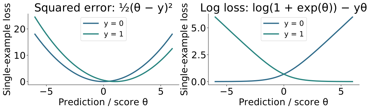
Logistic loss has flatter tails than squared error

• Each curve is the loss for one example, with its label fixed at \(y=0\) or \(y=1\).
• Squared error has constant curvature; log loss flattens toward a confident correct prediction.
• For \(y=1\), log loss decreases as the score grows; for \(y=0\), it decreases as the score falls.

Analytic per-example curves, not an average over conflicting labels. For squared error theta is the numerical prediction; for logistic loss theta is the pre-sigmoid score. Vertical scales differ. A dataset objective averages its examples’ loss curves; its shape depends on their inputs and labels. Separable data need not give a finite minimizer. No coefficient penalty is used.

A derivative predicts the effect of a small parameter change

First-order Taylor expansion centered at \(\theta\), for a small change \(\Delta\):

\[J(\theta+\Delta)\approx J(\theta)+J'(\theta)\Delta.\]

• If \(J'(\theta)>0\), a small negative change reduces the objective.
• If \(J'(\theta)<0\), a small positive change reduces it.
• This is a local approximation, not a prediction for an arbitrary step.

Three minutes. Bridge familiar scalar derivatives to their computational role. Theta is an illustrative scalar parameter, not a random variable. Draw a tangent line and explain what “small” means geometrically. The learning-rate issue follows.

A gradient collects the partial derivatives

Bundle the parameters into \(\boldsymbol{\theta}=(w_1,\ldots,w_d,b)^{\mathsf T}\).

\[ \nabla J(\boldsymbol{\theta})= \begin{bmatrix} \partial J/\partial w_1 & \cdots & \partial J/\partial w_d & \partial J/\partial b \end{bmatrix}^{\mathsf T}. \]

For a small vector change \(\boldsymbol{\Delta}\):

\[J(\boldsymbol{\theta}+\boldsymbol{\Delta}) \approx J(\boldsymbol{\theta})+\nabla J(\boldsymbol{\theta})^{\mathsf T}\boldsymbol{\Delta}.\]

The gradient has one component per parameter.

Three minutes. Each partial derivative changes one parameter while fixing the others. Connect shapes to Arc 2: the inner product produces one scalar predicted change in the objective. Different feature scales change gradient magnitudes.

Moving against the gradient gives local descent

For \(\alpha>0\), choose \(\boldsymbol{\Delta}=-\alpha\nabla J(\boldsymbol{\theta})\).

\[ \nabla J(\boldsymbol{\theta})^{\mathsf T}\boldsymbol{\Delta} =-\alpha\|\nabla J(\boldsymbol{\theta})\|_2^2\le0. \]

This motivates the repeated update

\[\boldsymbol{\theta}_{t+1}=\boldsymbol{\theta}_t-\alpha\nabla J(\boldsymbol{\theta}_t).\]

Next: inspect what these finite steps do when we can see only the local slope.

Three minutes. Strictly negative when the gradient is nonzero. The inequality concerns the first-order predicted change; a finite step can still increase the actual objective. For the convex objectives just established, a zero gradient establishes global optimality; a finite step still needs an appropriate learning rate. Do not skip the derivative of sigmoid/log loss when deriving the logistic update next class. Numerical convergence and generalization remain separate.

Small steps follow the local downhill direction

Same objective, same starting point. Learning rate: \(\alpha=2.0\).

The algorithm sees this point and this slope.

A negative-gradient step uses that local information.

Gold segments show only the slopes we have evaluated.

The objective falls; the slope keeps its sign.

Three steps approach the minimum.

Two minutes. Initial state: one point and tangent, no curve. Click 1 animates the first update and reveals the answer; click 2 reveals the next update; click 3 the final landing; click 4 reveals the entire curve. Exactly three tangent segments are accumulated, at theta_0, theta_1, theta_2, with a final landing point theta_3. The dashed connectors show jumps, not an evaluated path or the objective curve. Axes are scaled separately for readability; do not compare visual steepness across slides.

The same unregularized logistic objective is used throughout: J(theta)=log(1+exp(theta))-theta/2. Two observations have x=1, labels 0 and 1, score theta, no separate intercept. Its derivative is sigmoid(theta)-1/2. The stationary minimum is theta=0; curvature is at most 1/4 and tends to zero in the tails. Alpha=2 gives a monotone approach; alpha=6 gives shrinking alternating steps; alpha=12 increases loss on the first step, then keeps oscillating and a bounded nonzero two-cycle in the long run. This is failure to converge, not unbounded divergence. No penalty is needed. A finite-data logistic objective has bounded gradients; do not describe the first few rising losses as a proof of unbounded divergence.

Step	theta	objective	slope
0	2.000	1.127	+0.381
1	1.238	0.874	+0.275
2	0.688	0.751	+0.165
3	0.357	0.709	+0.088

\(\theta_{t+1}=\theta_t-\alpha J'(\theta_t)\) · Unregularized logistic loss · Three updates; the first three evaluated slopes remain visible.

What happens after this larger step?

Same objective, same starting point. Learning rate: \(\alpha=6.0\).

After the next update, what happens?

A. Objective decreases; slope keeps its sign.
B. Objective decreases; slope reverses sign.
C. Objective increases; slope keeps its sign.
D. Objective increases; slope reverses sign.

B. The objective falls, but the slope reverses: we jumped across the valley.

Three steps approach the minimum.

Three minutes including the four-choice question; instructor explicitly overrides the three-choice guidance. Initial state: one point and tangent, no curve. Click 1 animates the first update and reveals the answer; click 2 reveals the next update; click 3 the final landing; click 4 reveals the entire curve. Exactly three tangent segments are accumulated, at theta_0, theta_1, theta_2, with a final landing point theta_3. The dashed connectors show jumps, not an evaluated path or the objective curve. Axes are scaled separately for readability; do not compare visual steepness across slides.

The same unregularized logistic objective is used throughout: J(theta)=log(1+exp(theta))-theta/2. Two observations have x=1, labels 0 and 1, score theta, no separate intercept. Its derivative is sigmoid(theta)-1/2. The stationary minimum is theta=0; curvature is at most 1/4 and tends to zero in the tails. Alpha=2 gives a monotone approach; alpha=6 gives shrinking alternating steps; alpha=12 increases loss on the first step, then keeps oscillating and a bounded nonzero two-cycle in the long run. This is failure to converge, not unbounded divergence. No penalty is needed. A finite-data logistic objective has bounded gradients; do not describe the first few rising losses as a proof of unbounded divergence.

Step	theta	objective	slope
0	2.000	1.127	+0.381
1	-0.285	0.703	-0.071
2	0.140	0.696	+0.035
3	-0.069	0.694	-0.017

\(\theta_{t+1}=\theta_t-\alpha J'(\theta_t)\) · Unregularized logistic loss · Three updates; the first three evaluated slopes remain visible.

What happens when we take an even larger step?

Same objective, same starting point. Learning rate: \(\alpha=12.0\).

After the next update, what happens?

A. Objective decreases; slope keeps its sign.
B. Objective decreases; slope reverses sign.
C. Objective increases; slope keeps its sign.
D. Objective increases; slope reverses sign.

D. The objective rises and the slope reverses: we jumped too far.

Continuing these updates settles into an oscillation instead of reaching the minimum.

Three minutes including the four-choice question; instructor explicitly overrides the three-choice guidance. Initial state: one point and tangent, no curve. Click 1 animates the first update and reveals the answer; click 2 reveals the next update; click 3 the final landing; click 4 reveals the entire curve. Exactly three tangent segments are accumulated, at theta_0, theta_1, theta_2, with a final landing point theta_3. The dashed connectors show jumps, not an evaluated path or the objective curve. Axes are scaled separately for readability; do not compare visual steepness across slides.

The same unregularized logistic objective is used throughout: J(theta)=log(1+exp(theta))-theta/2. Two observations have x=1, labels 0 and 1, score theta, no separate intercept. Its derivative is sigmoid(theta)-1/2. The stationary minimum is theta=0; curvature is at most 1/4 and tends to zero in the tails. Alpha=2 gives a monotone approach; alpha=6 gives shrinking alternating steps; alpha=12 increases loss on the first step, then keeps oscillating and a bounded nonzero two-cycle in the long run. This is failure to converge, not unbounded divergence. No penalty is needed. A finite-data logistic objective has bounded gradients; do not describe the first few rising losses as a proof of unbounded divergence.

Step	theta	objective	slope
0	2.000	1.127	+0.381
1	-2.570	1.359	-0.429
2	2.577	1.362	+0.429
3	-2.575	1.361	-0.429

\(\theta_{t+1}=\theta_t-\alpha J'(\theta_t)\) · Unregularized logistic loss · Three updates; the first three evaluated slopes remain visible.

The gradient is an average of example contributions

If \(J(\boldsymbol{\theta})=\frac1n\sum_i\ell_i(\boldsymbol{\theta})\), then

\[\nabla J(\boldsymbol{\theta})=\frac1n\sum_i\nabla\ell_i(\boldsymbol{\theta}).\]

Update	Examples used for one gradient estimate
Full-batch GD	All \(n\) examples
Single-example SGD	One randomly sampled example
Mini-batch SGD	A small randomly sampled group \(B\)

All use \(\boldsymbol{\theta}_{t+1}=\boldsymbol{\theta}_t-\alpha_t\boldsymbol{g}_t\).

Minibatch is the intended third category; batchGD conventionally means fullbatch. With a fixed regularizer, add its gradient once to each estimate, not once per sampled loss without normalization.

Sampling trades exact direction for cheaper, noisy updates

For uniform sampling at the current parameters:

\[\boldsymbol{g}_B=\frac1{|B|}\sum_{i\in B}\nabla\ell_i(\boldsymbol{\theta}), \qquad \mathbb E_B[\boldsymbol{g}_B\mid\boldsymbol{\theta}]=\nabla J(\boldsymbol{\theta}).\]

• One stochastic step can increase the full training objective.
• Larger batches usually reduce gradient noise but cost more per update.
• Compare runs by examples processed or time, not only update count.

A fixed learning rate can leave persistent fluctuations near the minimum.

Uniform independent draws or a uniformly chosen subset give the unbiased mean at fixed theta. Sequential random reshuffling has a more nuanced conditional statement. Declining step sizes can improve settling under appropriate conditions.

Adam averages directions and adapts the step size for each parameter

For the current gradient estimate \(\boldsymbol{g}_t\):

\[\boldsymbol{m}_t=\beta_1\boldsymbol{m}_{t-1}+(1-\beta_1)\boldsymbol{g}_t, \qquad \boldsymbol{v}_t=\beta_2\boldsymbol{v}_{t-1}+(1-\beta_2)\boldsymbol{g}_t^2.\]

The hats correct the initial bias from \(\boldsymbol m_0=\boldsymbol v_0=\boldsymbol 0\): \[\widehat{\boldsymbol m}_t=\frac{\boldsymbol m_t}{1-\beta_1^t},\qquad \widehat{\boldsymbol v}_t=\frac{\boldsymbol v_t}{1-\beta_2^t}.\]

\[\boldsymbol{\theta}_{t+1}=\boldsymbol{\theta}_t- \alpha\frac{\widehat{\boldsymbol{m}}_t}{\sqrt{\widehat{\boldsymbol{v}}_t}+\epsilon}.\]

Average the recent directions; reduce the step size for parameters with large recent squared gradients.

The base learning rate still matters. Adaptation is not a convergence guarantee.

source:kingma-ba-adam. Elementwise square/root/division. Initialize m0=v0=0; hats correct initial bias: mhat=mt/(1-beta1^{t),vhat=vt/(1-beta2}t). beta values weight history; epsilon prevents division by zero. Do not teach an optimizer catalog or transfer vanilla convex-GD guarantees to Adam. AdamW is a later optional note on decoupled weight decay.

The logistic objective has a directly computable gradient

Include the intercept in \(\widetilde{\boldsymbol x}_i=(\boldsymbol x_i^{\mathsf T},1)^{\mathsf T}\) and \(\boldsymbol\theta=(\boldsymbol w^{\mathsf T},b)^{\mathsf T}\); let \(a_i=\sigma(\boldsymbol\theta^{\mathsf T}\widetilde{\boldsymbol x}_i)\).

\[J(\boldsymbol\theta)=-\frac1n\sum_{i=1}^n\big[y_i\log a_i+(1-y_i)\log(1-a_i)\big],\qquad \nabla_{\boldsymbol\theta}J=\frac1n\sum_{i=1}^n(a_i-y_i)\widetilde{\boldsymbol x}_i.\]

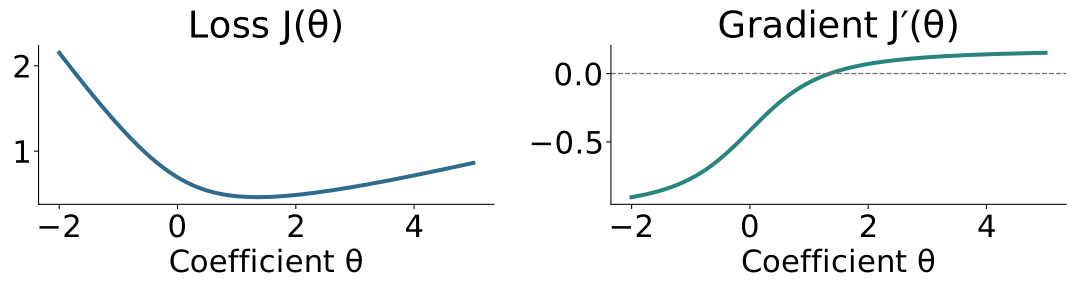
One-coefficient example: \(a_i=\sigma(\theta x_i)\), no intercept; \(J'(\theta)=\frac1n\sum_i(\sigma(\theta x_i)-y_i)x_i\).

Direct result of elementary chain rule and algebra; omit intermediate sigmoid and log derivatives. Vector theta contains d+1 parameters and gradient has the same dimension. The figure uses x=(-2,-1,-.5,.5,1,2), y=(0,0,1,0,1,1), no intercept and no penalty. All inputs are distinct. Solid curves show actual mean log loss and its analytic derivative. The next convergence experiment also fits an intercept. Use the gradient sign and zero crossing to connect the panels.

Each example contributes prediction error times its input

\[\nabla J(\boldsymbol\theta)=\frac1n\sum_i\underbrace{(a_i-y_i)}_{\text{probability residual}}\widetilde{\boldsymbol x}_i, \qquad \boldsymbol\theta_{t+1}=\boldsymbol\theta_t-\alpha\nabla J(\boldsymbol\theta_t).\]

• Underpredict a positive label: \(a_i-y_i<0\); that example’s descent contribution raises its score.
• Overpredict a negative label: \(a_i-y_i>0\); its descent contribution lowers its score.
• Average these contributions: examples can pull in different directions; larger feature values amplify the corresponding gradient entry.

Now watch the full training objective change over repeated updates.

For a single example, the score change from its descent contribution is proportional to -(a-y)||xtilde||^2. In a batch, other examples can counteract it; do not claim every example improves on each full-batch update. The intercept contribution uses the appended input 1. Learning rate controls the size of the combined step. No penalty or intermediate calculus derivation here.

Return to logistic regression and watch the fit evolve

Small illustrative dataset: six inputs \(x=(-2,-1,-0.5,0.5,1,2)\) and labels \(y=(0,0,1,0,1,1)\).

\[a_i=\sigma(wx_i+b),\qquad J(w,b)=\frac16\sum_i\ell(y_i,a_i).\]

Start every run at \((w,b)=(-0.5,0.8)\) and change only the learning rate.

The overlapping labels give a finite minimum without a coefficient penalty.

This six-point dataset is explicitly illustrative, not a subset of review data. Reference solution computed with BFGS to high accuracy; curves are actual full-batch GD runs. No regularization is used.

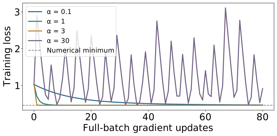
A linear loss axis shows large early improvements

Small steps are slow; larger useful steps improve quickly; oversized steps can keep oscillating.

Reference is a numerical minimum, not held-out error. The oversized-step trajectory fails to approach the minimum; the plot includes its full range. Same initialization and data for all learning rates.

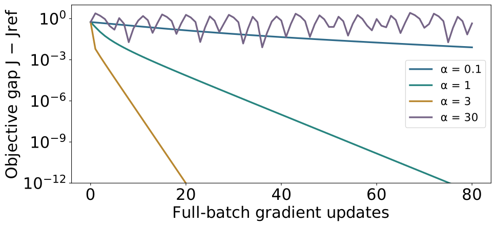
A log gap axis reveals progress near the minimum

Equal vertical distances now represent multiplicative changes in \(J-J_{\mathrm{ref}}\).

Jref is high-accuracy numerical reference, not an analytic answer or true population loss. Positive gaps below1e-14 are floored only for plotting; displayed lower range1e-12 avoids interpreting roundoff as progress. The oversized-step run has a persistent objective gap.

Convergence means little useful optimization remains

Check both a small gradient and small sustained changes in the objective.

• A visually flat trace alone may reflect a tiny learning rate or poor scaling.
• With a finite convex optimum, solving to useful tolerance is a sensible stopping point.
• Optimization progress is measured on training loss; generalization needs held-out evidence.

Near-zero loss does not automatically mean “finished”: separable logistic fits and large deep models need more care.

Do not claim a small gradient universally gives a tight distance-to-optimum bound without curvature assumptions. A strong-convexity bound can make that quantitative, but is beyond this introduction. Keep deep-model preview brief; neither zero loss nor further training guarantees good generalization.

Better optimization cannot repair the wrong function class

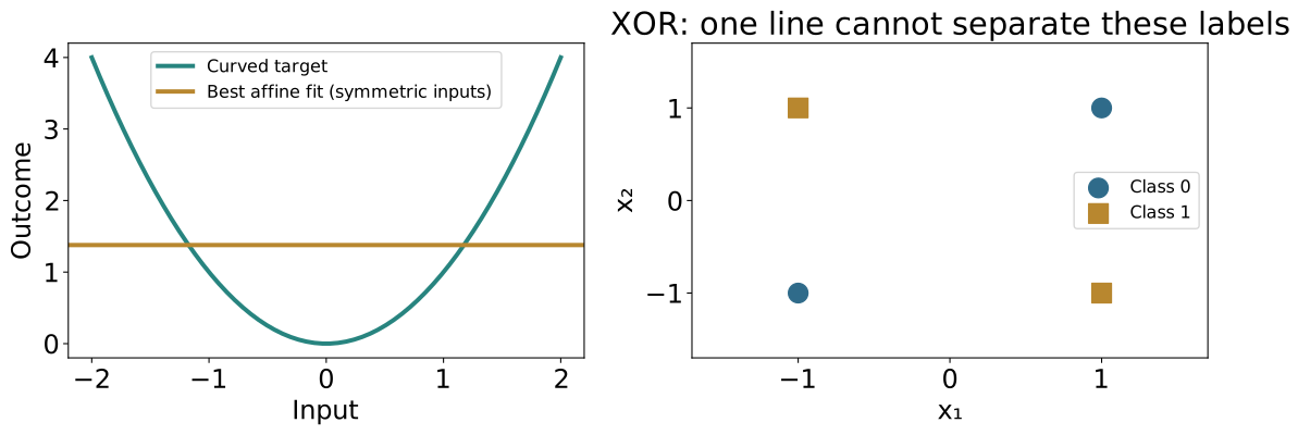
A curved numerical pattern and XOR labels cannot be represented by one affine predictor.

Illustrative analytic examples. Left line is leastsquares for symmetric inputs with squared target. Right contradictory inequalities show no affine classifier separates XOR; optional board proof using average of each class at origin. Distinguish representation failure from an unfinished fit.

The next arc changes the function we can represent

We now have: models → objectives → exact or numerical fitting → evaluation.

The remaining limitation: a single affine map cannot express every useful pattern.

Next task: categorize real product images. Can learned nonlinear features improve the predictor?

We will use XOR to explain the mechanism, then return to the real images.

30-second closing handoff to Arc5. No deep-learning machinery required before this point.