Learning Nonlinear Representations
A product image must become a useful category
A catalog task: assign a product image to a category such as shirt, bag, or shoe.
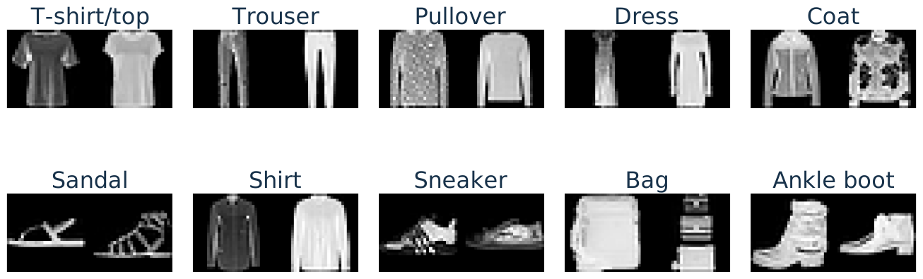
Fashion-MNIST: \(28\times28\) grayscale images, 784 pixel features , ten categories.
Zalando Research, Fashion-MNIST
About two minutes. [Sources] source:fashion-mnist; source:fashion-mnist-train-images; source:fashion-mnist-train-labels. These are actual product images, not generated illustrations. The benchmark contains 60,000 official training images and 10,000 test images. The figure uses the first two images of each class in our fixed training subset, without choosing examples using predictions. Ask students to notice variation within a category and resemblance across categories as an informal observation, not an additional live poll. Product catalog classification motivates the task, but this clean, low-resolution, single-item benchmark does not establish production performance on arbitrary seller photos, backgrounds, or unknown categories. Full benchmark classes are retained; do not select an easy or difficult binary pair after looking at results.
Softmax and cross-entropy extend binary logistic regression
For image \(\boldsymbol x\in[0,1]^{784}\) and category \(c=1,\ldots,10\) :
1. Compute a linear score: \(s_c=\boldsymbol w_c^{\mathsf T}\boldsymbol x+b_c\) .
2. Apply softmax to turn the scores into probabilities that sum to one:
\[p_c=\frac{\exp(s_c)}{\sum_{j=1}^{10}\exp(s_j)}.\]
3. Use cross-entropy: if the true category is \(y\) , penalize low \(p_y\) :
\[\ell(y,\boldsymbol p)=-\log p_y,\qquad J=\frac1n\sum_{i=1}^n-\log p_{i,y_i}.\]
Softmax generalizes sigmoid; cross-entropy generalizes binary log loss.
About three minutes. Define p_c as the probability assigned to category c for this image, y as its true category index, and p_{i,y_i} as example i’s probability for its true category. Predict the largest probability, equivalently the largest score. Average cross-entropy is the unpenalized data objective; the next slide fits candidates with an L2 weight penalty as in the prior regularization section. No one-hot notation is needed. In the two-class case p_1=sigma(s_1-s_2), so fixing one reference score recovers the earlier sigmoid model. For a one-hot true label, multiclass cross-entropy is exactly -log p_y; the binary expression -y log a-(1-y)log(1-a) selects the same true-label probability. Subtract the maximum score in numerical softmax implementations. Although the probabilities are nonlinear in x, pairwise decision boundaries s_c=s_j remain affine: the linear classifier terminology refers to its scores and boundaries. Do not call a sigmoid or softmax alone a learned nonlinear feature representation. [Sources] source:fashion-mnist; source:d2l-multilayer-perceptrons. Flattening and division by255 retain the image information. The same ten-score probability/loss construction is reused after hidden features later.
Regularization helps, but a nonlinear model improves validation accuracy
Same 12,000 training and 3,000 validation images; same pixel features.
Linear, \(C=0.01\) (stronger penalty)
84.66%
82.37%
Linear, \(C=0.1\)
88.70%
84.03%
Linear, \(C=1\)
92.21%
82.73%
Linear, \(C=10\) (weaker penalty)\(^*\)
94.90%
80.40%
Nonlinear model 94.10%
85.70%
\(C\) is inverse regularization strength. \(^*\) This fit reached its iteration limit.
How do we go beyond linear functions, and why can that help?
A tiny image task will make the missing interaction explicit.
About two minutes. [Sources] source:fashion-mnist; source:fashion-mnist-train-images; source:fashion-mnist-train-labels. These are the actual candidate results in fashion-mnist-results.json, not test accuracies. C is sklearn’s inverse penalty parameter: increasing C weakens regularization. Do not identify C numerically with the earlier lambda. The first three linear fits converged; C10 reached1500 iterations, is explicitly flagged, and was not selected. As the penalty weakens, training accuracy rises while validation need not improve. Among the tried linear settings, C0.1 is selected by validation. The nonlinear row is a one-hidden-layer 64-ReLU MLP with alpha0.01, selected among .0001,.01,1; architecture and 60-epoch Adam budget were fixed beforehand. Defer its internals until after XOR. Its training budget is not a convergence claim. Validation-selected accuracy is used to motivate/model-select, not as an unbiased final estimate; the later comparison uses official test data. No test outcomes were used for these choices. The observed gap motivates investigating learned features; it does not prove that every linear model must be worse, nor that the real dataset is literally XOR. Distinguish nonlinear probabilities from nonlinear scores, as on the preceding slide.
An image label can depend on relationships between regions
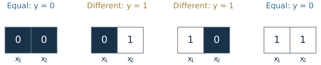
To isolate the mechanism, use a toy image task: flag a mismatch between two regions.
Represent their brightness by \(\boldsymbol{x}=[x_1,x_2]^{\mathsf T}\in\{0,1\}^2\) .
Predict \(y=1\) when the regions differ; otherwise predict \(y=0\) .
Bridge from the real product-image task to an exact, deliberately tiny example. This is an original two-pixel illustration, not a Fashion-MNIST sample or an empirical claim. Dark means0 and bright means1. Each square can also stand for one measured image region. The exact four cases are the complete task; no train/test performance is claimed. About two minutes. [Sources] source:d2l-multilayer-perceptrons, section5.1.1.1 motivates context-dependent image features; the construction and figures are original.
A raw linear score gives each pixel one fixed contribution
\[z=w_1x_1+w_2x_2+b,\qquad a=\sigma(z).\]
Changing \(x_1\) from 0 to 1 changes the score by \(w_1\) \(x_2\) is.
\(x_2=0\) Class changes from 0 to 1
\(x_2=1\) Class changes from 1 to 0
A monotone sigmoid cannot make the same score increment point both ways.
This is a limitation of this model on the defined XOR task, not a claim that all image tasks defeat linear predictors. Use the usual probability threshold1/2, equivalent to score threshold zero. A nonzero fixed w1 raises both scores or lowers both scores; zero changes neither. The sigmoid changes the magnitude of the probability response with context, but not its direction. About two minutes. [Sources] source:d2l-multilayer-perceptrons, section5.1.1.1. Original four-case argument.
XOR cannot be separated by one straight decision line
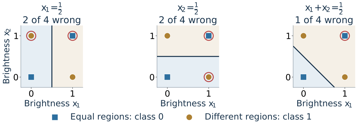
Toy image: two brightness features \(x_1,x_2\in\{0,1\}\) . Label different regions 1 , equal regions 0.
Shading shows predictions; markers show true classes. Red rings mark errors.
No single straight decision line separates the two classes.
About two minutes. Keep the preceding image setup and fixed-contribution explanation; this slide supplies the geometric intuition. Each panel predicts1 when w1x1+w2 x2+b>0: weights [1,0], [0,1], [1,1], with b=-1/2. Blue shading predicts0; gold predicts1. Filled squares/circles show true classes; red rings mark mistakes. Vertical and horizontal lines each miss two examples; the diagonal misses [1,1]. These candidate failures illustrate the limitation, rather than exhaustively testing every line. The previous slide supplies the general argument: changing x1 has the same signed effect on the linear score regardless of x2, whereas XOR requires opposite class changes. Moving or rotating one line cannot fix this. No additional geometric proof is needed here. [Sources] source:d2l-multilayer-perceptrons. Candidate constructions and figure are original.
A difference feature makes the same labels easy to separate
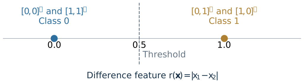
Choose the feature \(r(\boldsymbol{x})=|x_1-x_2|\) .
\[\widehat y=\mathbb 1\{r(\boldsymbol{x})>\tfrac12\}.\]
We changed the representation , not the four labels or the fitting algorithm.
About two minutes. Define the indicator as one when its condition is true and zero otherwise. The feature is hand chosen to expose the mechanism; do not imply it was learned. Feature maps can discard information: both equal-brightness images map to zero, which is appropriate for this task but not for every task. Next ask how to express such a feature using reusable trainable parts. [Sources] source:d2l-multilayer-perceptrons, section5.1.1.2 for learned representations; this absolute-difference construction is original.
A neuron applies a nonlinear function to a linear score
\[s=\boldsymbol{w}^{\mathsf T}\boldsymbol{x}+b,\qquad h=\phi(s).\]
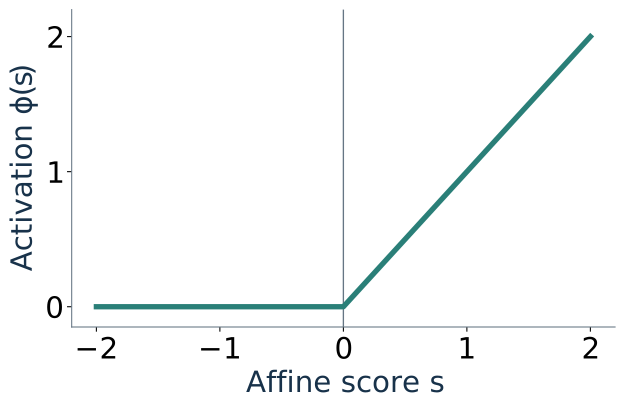
Rectified linear unit (ReLU):
\[\phi(s)=\max(0,s).\]
For \(\boldsymbol{w}=[1,-1]^{\mathsf T}\) and \(b=0\) :
\[h=\max(0,x_1-x_2).\]
It responds when region 1 is brighter.
About three minutes, including the examples [1,0] and [0,1]. We use phi for a hidden activation and reserve sigma for the already-known sigmoid. A neuron is a mathematical computation, not a detailed biological model. ReLU is continuous and piecewise linear, but not globally affine; it is nondifferentiable at zero. Hidden activations are not probabilities. The illustrative coefficients are selected by hand; training will eventually adjust them. [Sources] source:d2l-multilayer-perceptrons, sections5.1.1.3,5.1.2.1.
Two directional responses create a useful hidden representation
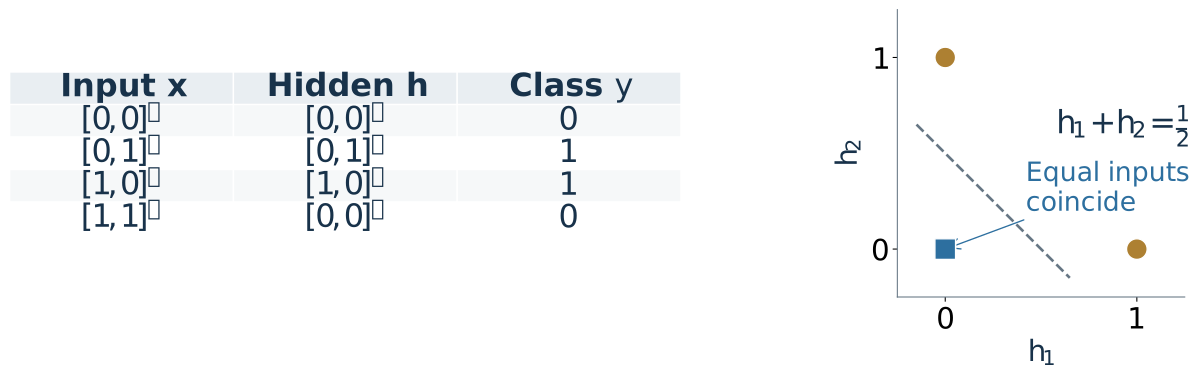
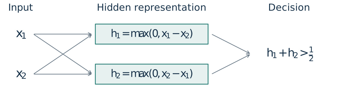
\[h_1=\max(0,x_1-x_2),\qquad h_2=\max(0,x_2-x_1).\]
\[h_1+h_2=|x_1-x_2|,\qquad \widehat y=\mathbb 1\{h_1+h_2>\tfrac12\}.\]
A linear decision in the hidden features solves the nonlinear input-space task.
About four minutes; work all four inputs using the arrows/table in the figure. Equal regions produce [0,0]; the two mismatch directions produce [1,0] and [0,1]. Hidden means an intermediate computed value, not an extra observed label. The sum is a linear output layer of nonlinear features. These hand-set weights establish representability only; they do not demonstrate successful training or generalization. Later training must fit the feature map and the output layer together. [Sources] source:d2l-multilayer-perceptrons, section5.1.1.2. Original exact construction.
A hidden layer collects several computed features into a vector
\[\boldsymbol{h}=[h_1,\ldots,h_m]^{\mathsf T}\in\mathbb R^m.\]
Each hidden unit has its own weights and bias; all see the same input.
The output layer combines the resulting features.
About two minutes. The diagram specializes to the two-unit example, with the two formulas inside their nodes so edges do not become an uninterpretable hairball. Generalize the number of hidden units to m. The dashed conceptual separation is representation versus output layer, not two separately fitted models. A dense layer allows every input-to-hidden connection even though a fitted weight could be zero. [Sources] source:d2l-multilayer-perceptrons, section5.1.1.2.
Stack the neuron weights to obtain one matrix expression
Each row of \(W\) is one neuron’s \(\boldsymbol w_j^{\mathsf T}\) :
\[\boldsymbol h=\phi(W\boldsymbol x+\boldsymbol b),\qquad
W\in\mathbb R^{m\times d},\quad \boldsymbol b\in\mathbb R^m.\]
Apply \(\phi\) separately to each feature.
For our two-region example:
\[W=\begin{bmatrix}1&-1\\-1&1\end{bmatrix},\quad
\boldsymbol b=\begin{bmatrix}0\\0\end{bmatrix},\quad
\boldsymbol h=\phi\!\left(\begin{bmatrix}x_1-x_2\\x_2-x_1\end{bmatrix}\right).\]
About two minutes. One observation is a column vector. Map each row to the neuron from the preceding diagram, rather than introducing a second orientation convention. Phi of a vector means elementwise ReLU; it is not matrix multiplication. Generic W and b are trainable, whereas the displayed example is an explicitly constructed setting. [Sources] source:d2l-multilayer-perceptrons, section5.1.1.3; translated to the course’s column-observation convention.
Dimensions account for every trainable parameter
One Fashion-MNIST image: \(784\) pixel features → \(64\) hidden units → \(10\) class scores.
\[\boldsymbol h=\operatorname{ReLU}(W\boldsymbol x+\boldsymbol b),\qquad
\boldsymbol s=V\boldsymbol h+\boldsymbol c.\]
Hidden layer
\(W:\ 64\times784\) \(\boldsymbol b:\ 64\times1\) \(64\cdot784+64=50{,}240\)
Output layer
\(V:\ 10\times64\) \(\boldsymbol c:\ 10\times1\) \(10\cdot64+10=650\)
Total: \(50{,}240+650=50{,}890\) trainable parameters.
Activations: \(\boldsymbol x\in\mathbb R^{784}\) , \(\boldsymbol h\in\mathbb R^{64}\) , \(\boldsymbol s,\boldsymbol p\in\mathbb R^{10}\) . Softmax converts scores \(\boldsymbol s\) to probabilities \(\boldsymbol p\) and adds no parameters .
About two minutes. [Sources] source:fashion-mnist; source:d2l-multilayer-perceptrons. These are the exact dimensions of the product-image experiment. One observation is a column vector, with no batch axis yet. W,b,V,c are all the trainable parameters; inputs, activations, scores, and probabilities are computed values, not additional parameters. ReLU and softmax have no trainable parameters. Fixed-order flattening preserves pixel values but a dense layer does not enforce spatial locality or weight sharing.
The output layer maps learned features to multiclass probabilities
For the product images, let \(\boldsymbol h\in\mathbb R^{64}\) and compute
\[\boldsymbol s=V\boldsymbol h+\boldsymbol c,\qquad V\in\mathbb R^{10\times64},\quad\boldsymbol c\in\mathbb R^{10}.\]
Reuse softmax to normalize the ten scores into class probabilities:
\[p_c=\frac{\exp(s_c)}{\sum_{j=1}^{10}\exp(s_j)},\qquad c=1,\ldots,10.\]
For class labels \(y_i\) , fit all parameters \(\boldsymbol\theta=(W,\boldsymbol b,V,\boldsymbol c)\) jointly using mean cross-entropy : \[J(\boldsymbol\theta)=-\frac1n\sum_i\log p_{i,y_i}.\]
About three minutes. Revisit the softmax/cross-entropy bridge introduced with the linear baseline. Only the learned input to the output layer changes: h replaces x. Binary sigmoid outputs one positive-class probability, whereas these ten mutually exclusive labels need one normalized distribution. Define p_c as the probability assigned to category c for this image and y as its class index. No one-hot encoding or softmax derivative is needed yet. Average this loss across training examples and add the selected L2 penalty. The linear baseline uses the same ten-score softmax output layer directly on x; the MLP inserts learned nonlinear h. The model is 784 -> 64 ReLU -> 10, with 50,890 parameters including the output layer. This is simpler to express using the matrix operations already taught; it is not claimed to use fewer parameters than every CNN. Numerical implementations subtract the largest score before exponentiating. [Sources] source:fashion-mnist; source:d2l-multilayer-perceptrons. Softmax is defined directly here as a normalized-exponential construction, not an unstated prerequisite.
Deeper models compose learned representations
\[\boldsymbol h^{(0)}=\boldsymbol x,\] \[\boldsymbol h^{(\ell)}=\phi_\ell\!\left(W_\ell\boldsymbol h^{(\ell-1)}+\boldsymbol b_\ell\right),
\qquad \ell=1,\ldots,k.\]
\[\boldsymbol x\ \longrightarrow\ \boldsymbol h^{(1)}\ \longrightarrow\ \boldsymbol h^{(2)}\ \longrightarrow\ \text{prediction}.\]
Each layer transforms features produced by the previous layer.
An MLP—multilayer perceptron—uses dense layers with nonlinear hidden activations.
About two minutes. Superscripts index layers, not powers; k here counts hidden layers. If consecutive widths are m_(ell-1) and m_ell, W_ell has shape m_ell by m_(ell-1). ReLU can be used at every hidden layer, while the output layer depends on the task. A learned feature need not have a neat human label; do not promise an automatic edge-to-object hierarchy. This establishes the composition vocabulary before backpropagation or convolution. [Sources] source:d2l-multilayer-perceptrons, sections5.1.1.2–5.1.1.3.
Composing linear layers still gives one linear layer
A linear layer computes \(W\boldsymbol x+\boldsymbol b\) (technically affine when \(\boldsymbol b\ne\boldsymbol 0\) ).
\(f(\boldsymbol x)\)
\(=\)
\(W_2(W_1\boldsymbol x+\boldsymbol b_1)+\boldsymbol b_2\)
(two linear layers)
\(\,\)
\(=\)
\(W_2W_1\boldsymbol x+W_2\boldsymbol b_1+\boldsymbol b_2\)
(distribute)
\(\,\)
\(=\)
\(A\boldsymbol x+\boldsymbol c\)
(\(A=W_2W_1\) , \(\boldsymbol c=W_2\boldsymbol b_1+\boldsymbol b_2\) )
Repeat this argument for any number of linear layers.
About three minutes. State compatible dimensions before expanding. The vector c here denotes the combined bias for a possibly vector-valued linear layer; it is the combined bias, not an extra trainable layer. A narrow hidden layer can restrict rank further, but never creates a nonlinear score. Keep the first complete equality visible initially and reveal one justified row at a time. [Sources] source:d2l-multilayer-perceptrons, section5.1.1.3; column-vector derivation.
More expressive features still need held-out evidence
Can this architecture express a useful rule?
A construction or approximation argument
Did training find useful parameters?
Training objective and optimization diagnostics
Does the fitted predictor work on new examples?
Appropriate held-out evaluation
Choose width, depth, and regularization using validation data; reserve test data for final assessment.
Our four-image construction answers only the first question.
About two minutes. Revisit the Arc3/4 evaluation contract. Training improvements do not prove transfer; a wider model can express more but may need different amounts of data and computation. Learned hidden features do not remove the need to choose inputs, architecture, or splits. Do not introduce a universal monotonic width-to-test-error relationship. The tiny deterministic truth table has no measured generalization claim.
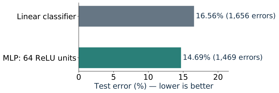
A small MLP makes fewer product-image errors in this experiment
187 fewer errors on 10,000 test images. Same inputs and split; each model selected on validation data.
About two minutes. [Sources] source:fashion-mnist; source:fashion-mnist-train-images; source:fashion-mnist-train-labels; source:fashion-mnist-test-images; source:fashion-mnist-test-labels. Reproduced locally with lectures/scripts/arc5_fashion_mnist.py, recorded in fashion-mnist-results.json. The official 60,000-image training pool supplies a stratified 15,000-image subset with seed570, then 12,000 fit / 3,000 validation; 45,000 are unused. Test data are the full official 10,000 examples. Pixel scale is /255 for both. Linear model C candidates .01,.1,1,10; selected .1 (validation84.03%, test83.44%) converged in451 iterations. The C10 candidate reached its iteration cap and was not selected. MLP architecture is fixed 784->64ReLU->10softmax, Adam step .001, batch256, 60 epochs, alpha candidates .0001,.01,1; selected .01 (validation85.70%, test85.31%). All MLP fits hit the deliberately fixed epoch budget; no convergence claim. No refit, augmentation, test-driven tuning, favorable-seed search, CNN, or transformer comparison. Absolute error reduction1.87 percentage points; relative error reduction about11.3%. This modest gain is evidence for this fitted model on this split, not proof that all linear models have a nonzero irreducible error or that an MLP wins every dataset. Hand-set XOR features explained the mechanism; these features were learned from real training images.