Training Neural Networks

Last updated October 16, 2026

David I. Inouye

We still use gradient descent—but where do the gradients come from?

\[\boldsymbol\theta\leftarrow\boldsymbol\theta-\eta\nabla_{\boldsymbol\theta}J.\]

The parameters now sit inside a composition of many layers.

Backpropagation computes \(\nabla_{\boldsymbol\theta}J\) efficiently. Gradient descent (or Adam) uses those gradients to update the parameters.

Training loop: forward computation → backpropagation → parameter update.

About two minutes. Start from the already familiar optimizer. Backpropagation is the differentiation algorithm, not a replacement for gradient descent. For a batch objective, differentiate its mean loss. The next slides use a single-example scalar loss to isolate the mechanism. Original calculus exposition.

Backpropagation evaluates the chain rule from the loss backward

For \(a=f(\theta)\), \(b=g(a)\), and \(\ell=q(b)\):

\[\frac{\partial\ell}{\partial\theta} =\frac{\partial\ell}{\partial b}\, \frac{\partial b}{\partial a}\, \frac{\partial a}{\partial\theta}.\]

Forward: \(\theta\to a\to b\to\ell\); save the values needed by the derivatives.

Backward: start with \(\frac{\partial\ell}{\partial\ell}=1\), then compute

\[\frac{\partial\ell}{\partial b}=\frac{\partial q(b)}{\partial b},\qquad \frac{\partial\ell}{\partial a}=\frac{\partial\ell}{\partial b}\,\frac{\partial b}{\partial a},\qquad \frac{\partial\ell}{\partial\theta}=\frac{\partial\ell}{\partial a}\,\frac{\partial a}{\partial\theta}.\]

Same chain rule, reversed evaluation order. We need the forward output to evaluate the loss’s derivative, and saved intermediate values to evaluate the local derivatives.

About three minutes. The flipped aspect is the direction of sensitivity propagation, not an inverse function and not a new calculus identity. For squared loss \(q(b)=\tfrac12(b-y)^2\), \(\partial q(b)/\partial b=b-y\) depends on the computed prediction b; merely knowing the label is insufficient. Backward is seeded with one because the derivative of the scalar loss with respect to itself is one. The numeric loss value itself need not be stored if its derivative can be evaluated from the prediction and target. Values can alternatively be recomputed, trading computation for memory. Reverse accumulation shares intermediate sensitivities across parameters instead of redoing the whole chain for each parameter.

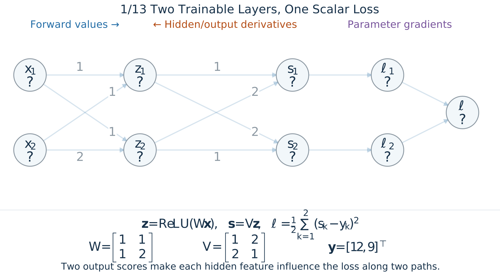
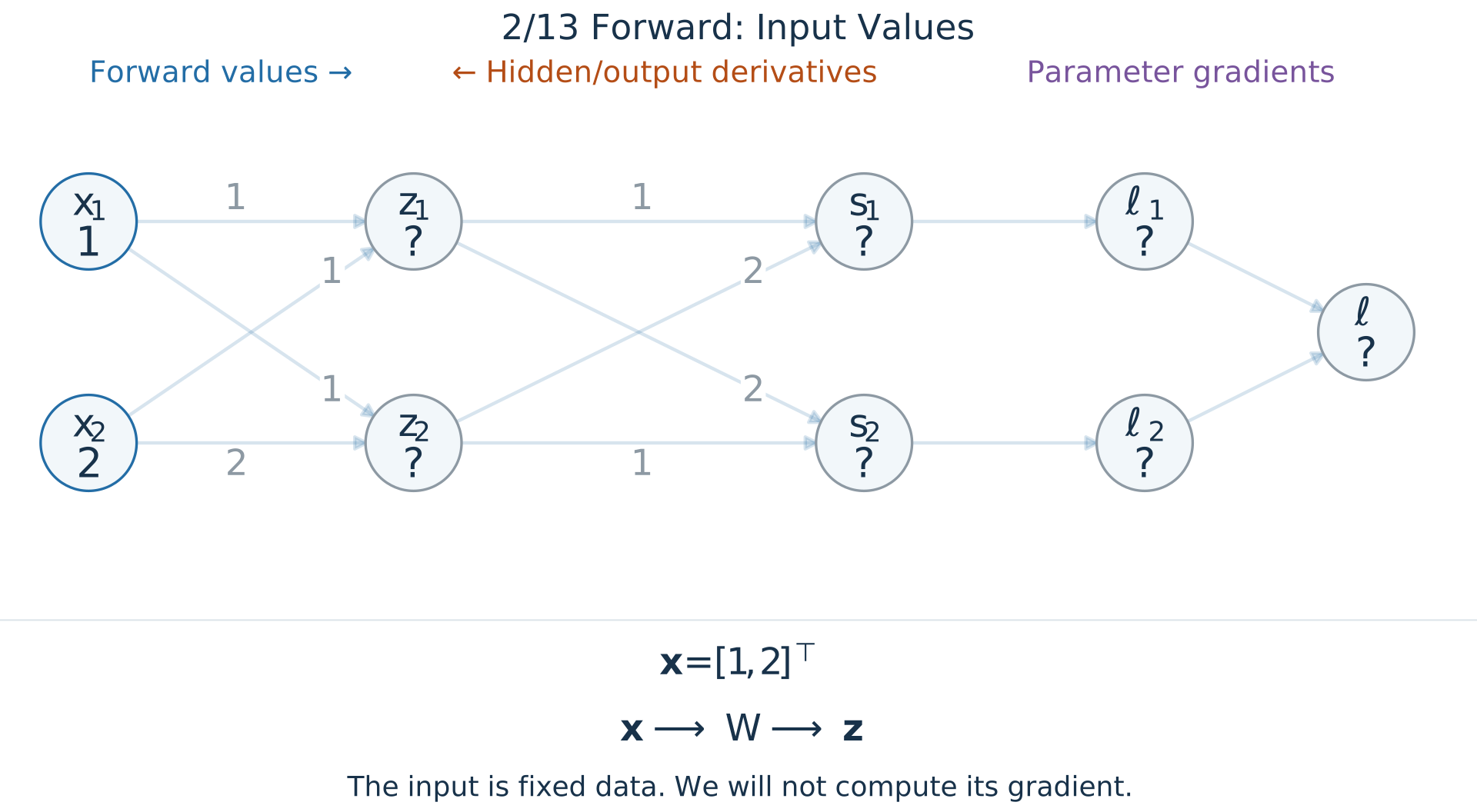
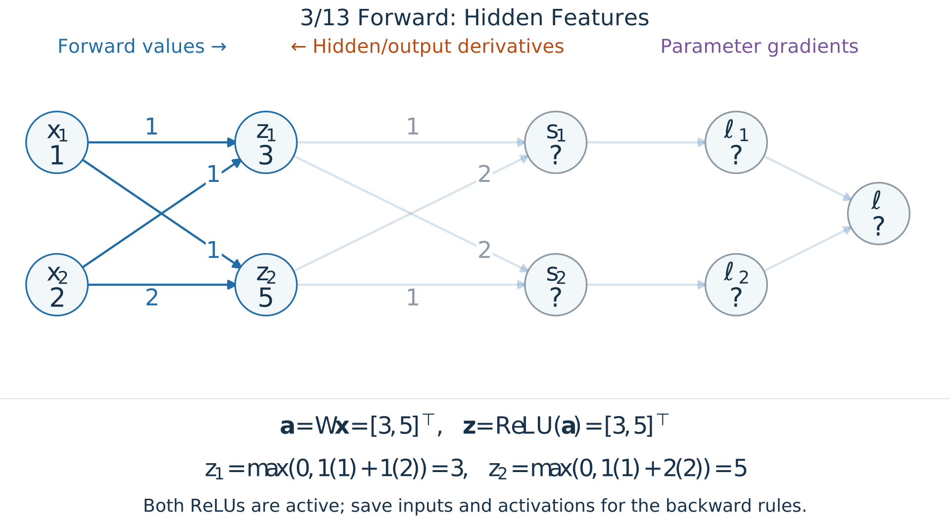
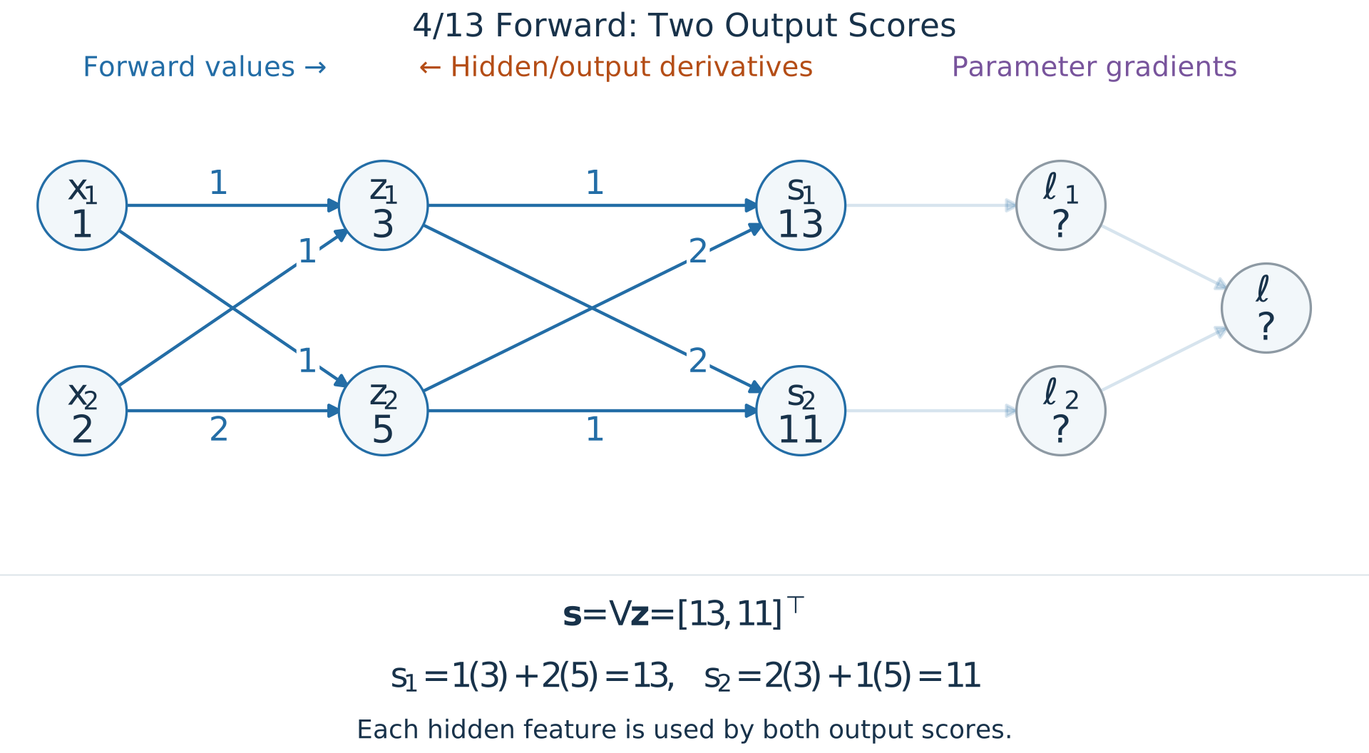
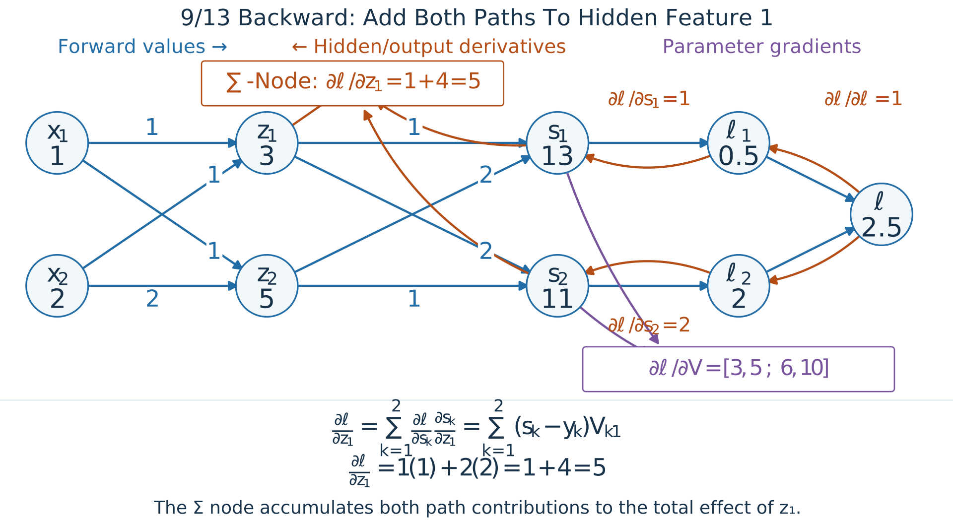
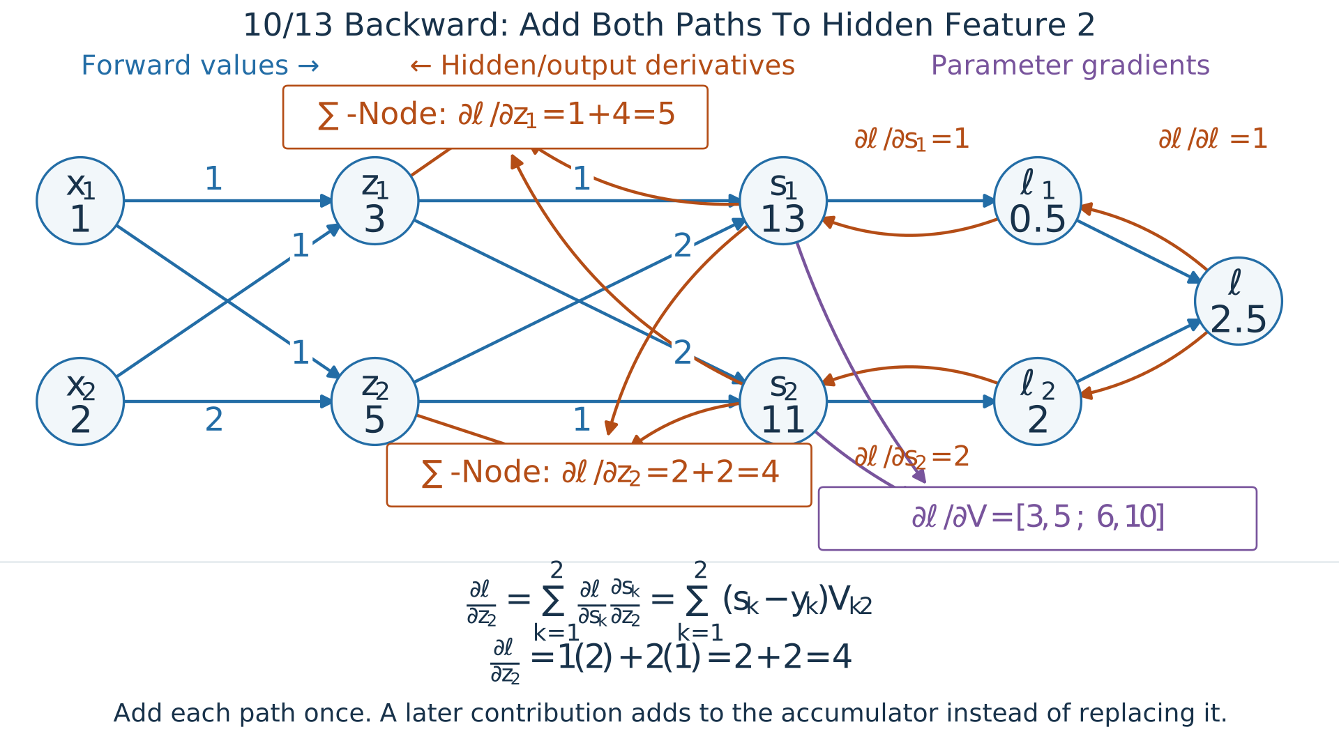
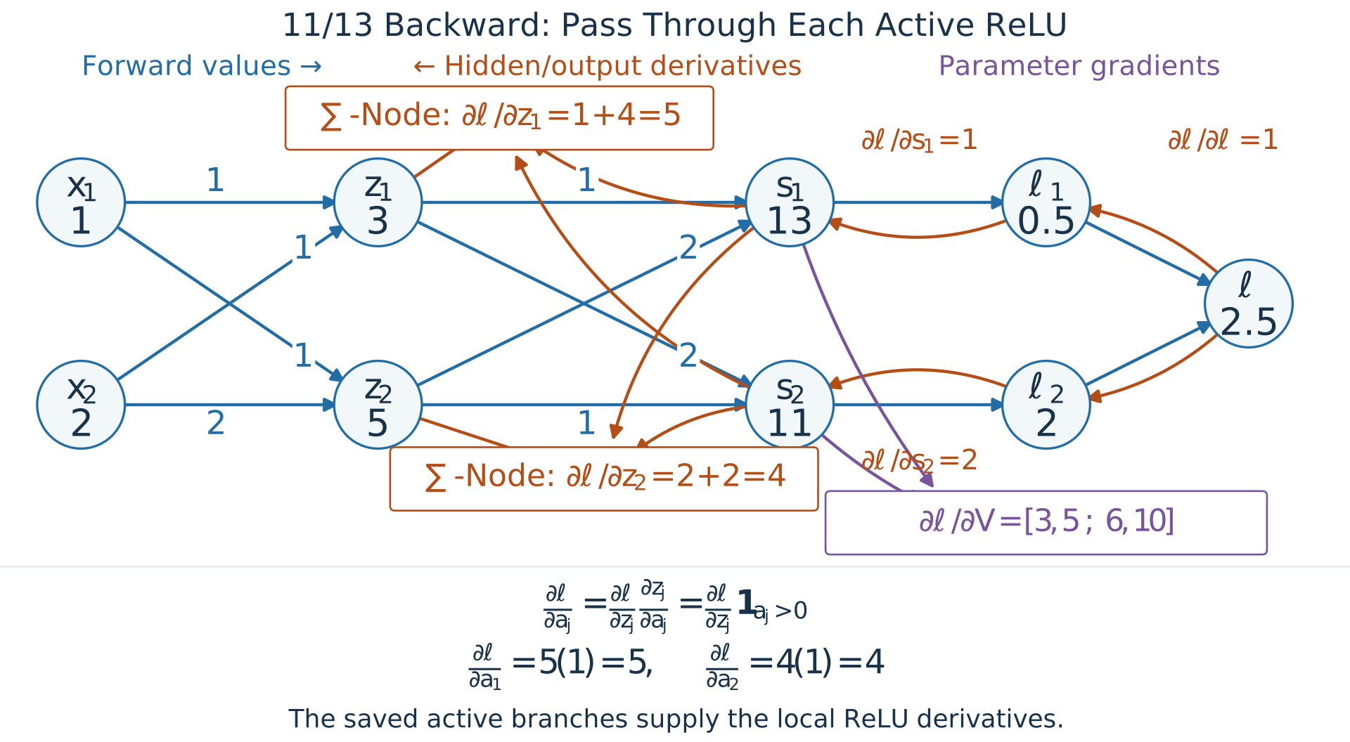
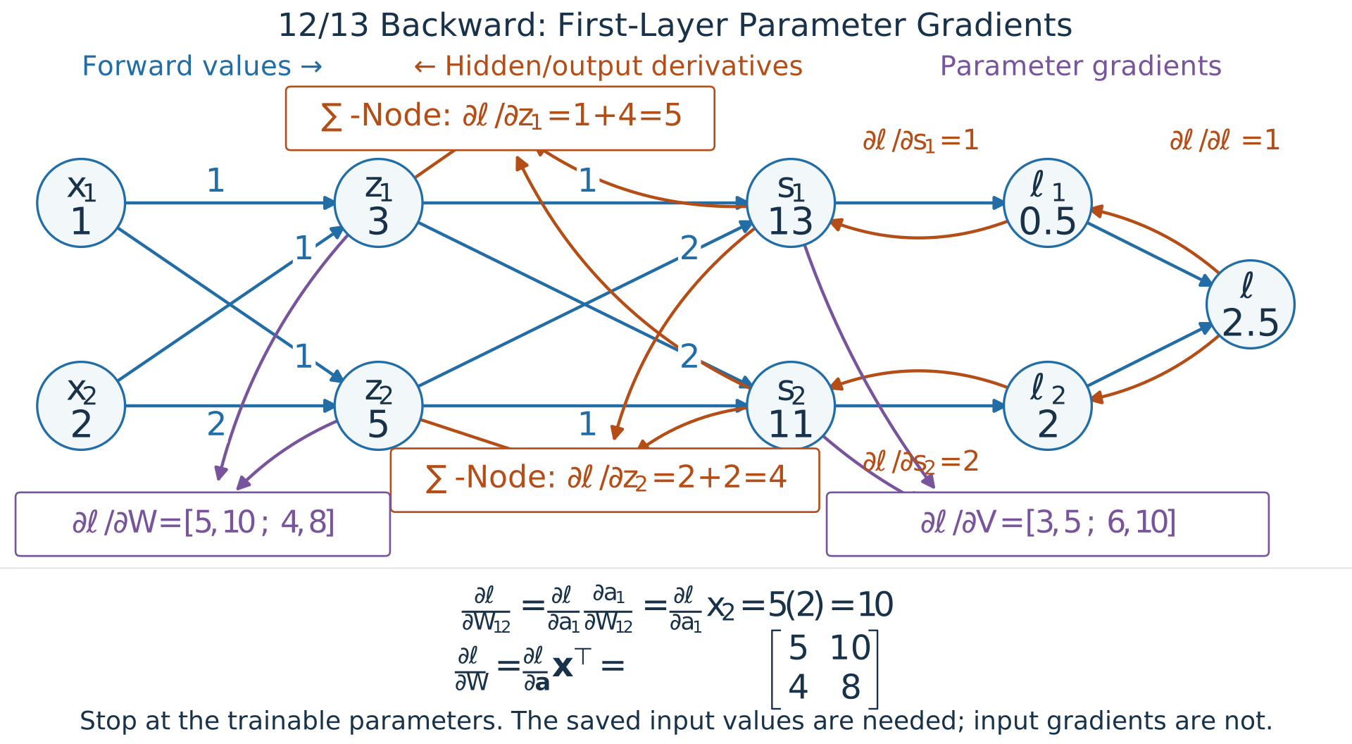
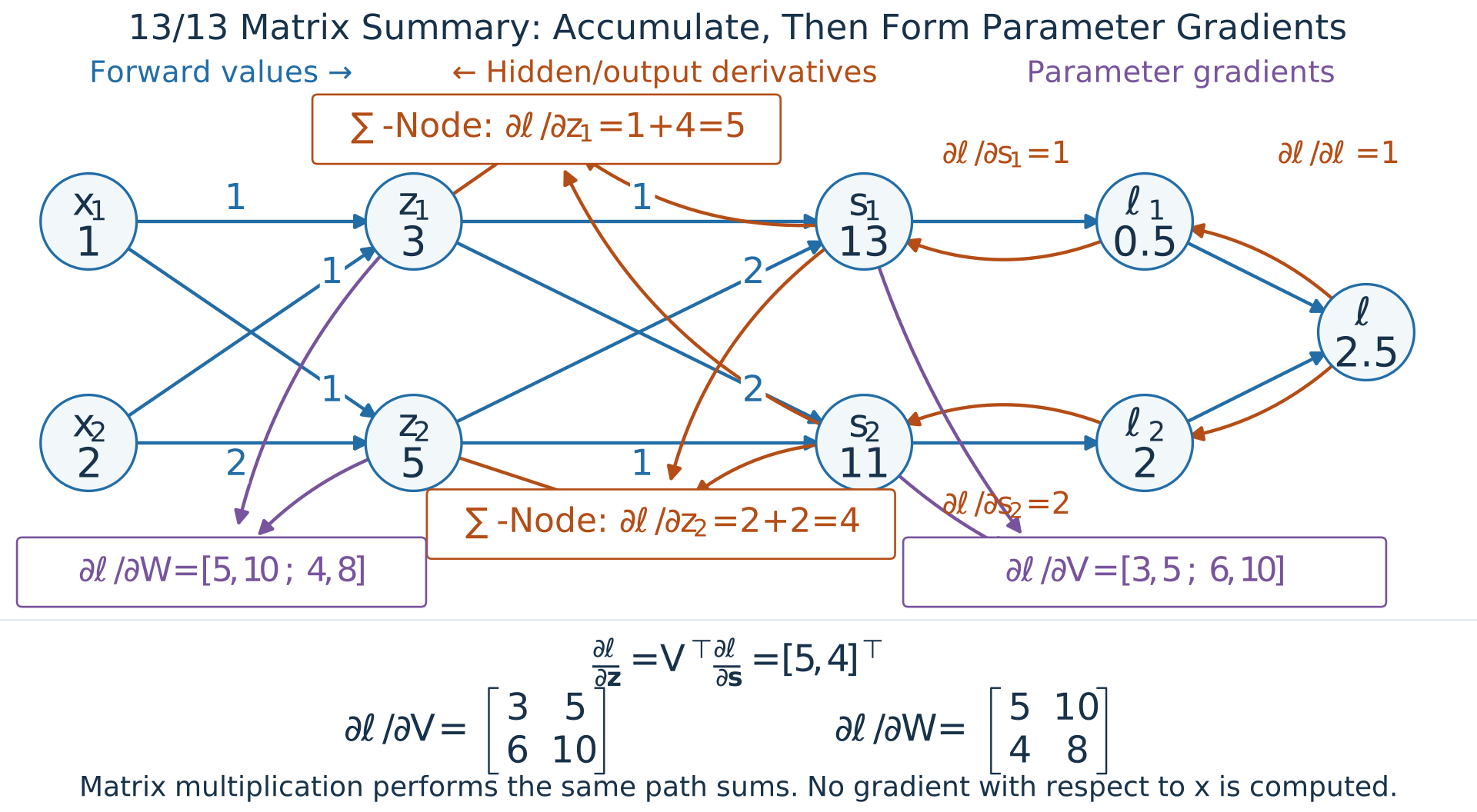
Backward computation sums paths at hidden features

About seven minutes for the complete thirteen-state walkthrough. Advance and rewind with normal Reveal controls; PDF shows the final summary. This is an original bias-free MLP with exactly two trainable linear layers: 2 inputs → 2 ReLU hidden features → 2 output scores, followed by one scalar sum of squared losses. x=[1,2], W rows [1,1] and [1,2], z=ReLU(a)=[3,5], V rows [1,2] and [2,1], s=[13,11], y=[12,9]. The two loss terms are 0.5 and 2; their sum is 2.5. PyTorch independently verifies every parameter and hidden derivative with x.requires_grad=False.

Every backward explanation starts with the full chain rule in partial derivatives, then substitutes the local forward-operation derivative symbolically, then evaluates the numbers. The loss sum passes one to each loss term. The score sensitivities are s-y=[1,2]. At each output, distinguish parameter gradients from sensitivities passed toward the hidden representation: partial ell / partial V is the outer product of the score sensitivities with saved z, giving rows [3,5] and [6,10].

Each hidden feature feeds both output scores. Its orange Sigma node accumulates the total effect over all paths: partial ell / partial z_j = sum_k (partial ell / partial s_k)(partial s_k / partial z_j) = sum_k (s_k-y_k)V_kj. For z_1, 11+22=5; for z_2, 12+21=4. These are total path contributions written as partial derivatives of the overall scalar loss with respect to one hidden value while holding the other hidden value fixed. The Sigma boxes are backward accumulators, not additional forward neurons. V transpose times the score sensitivities expresses the same sums in matrix form.

Both ReLUs are active, so the hidden-preactivation sensitivities remain [5,4]. First-layer parameter gradients use saved x values, producing W-gradient rows [5,10] and [4,8]. Stop here: ordinary supervised parameter training needs those input values but does not need gradients with respect to fixed x. No orange arrows go back to x and no parameter update occurs during backward. Compact gradient boxes separate matrix rows with a semicolon; the equations use conventional matrix layouts. This multi-output regression loss makes the branching structure transparent without adding a softmax Jacobian; Fashion-MNIST retains its cross-entropy objective.

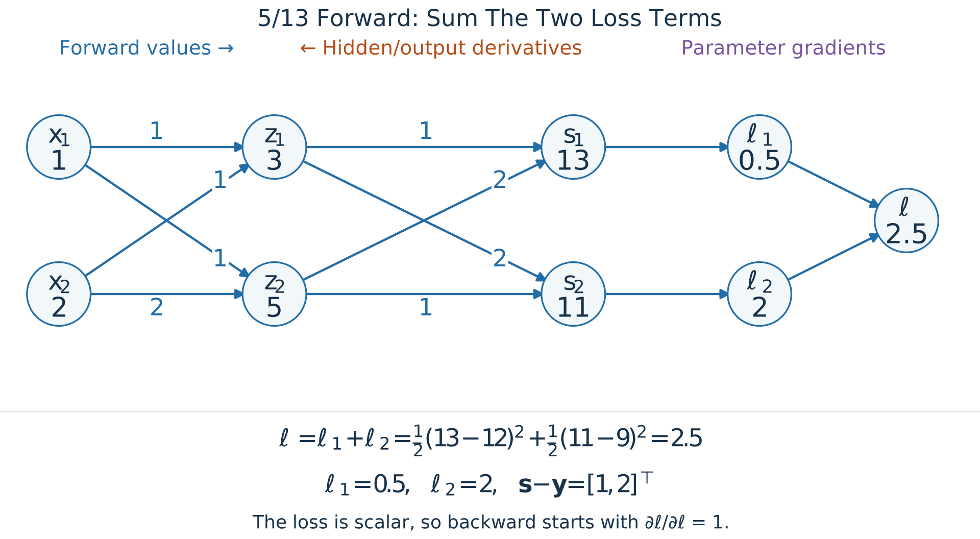
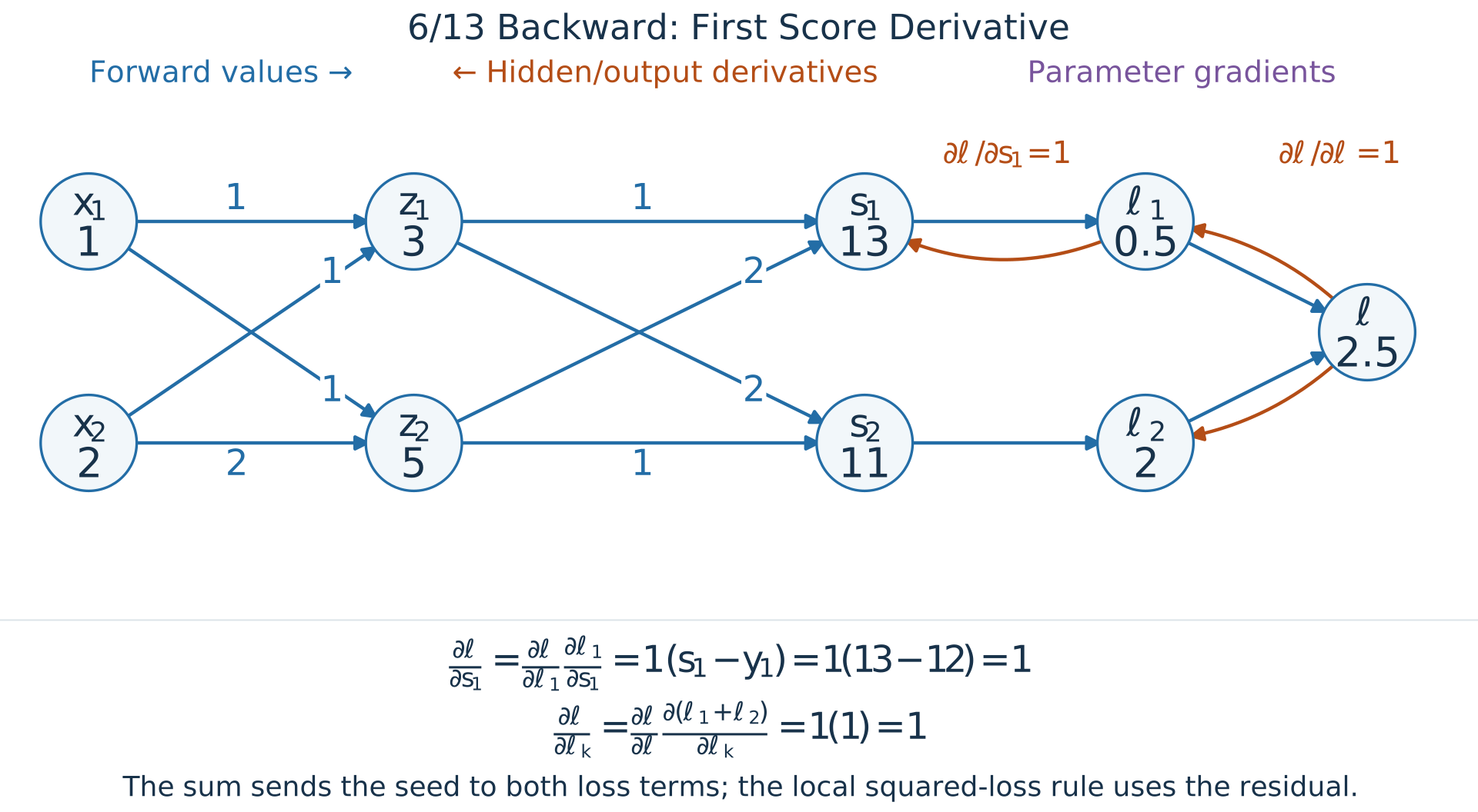
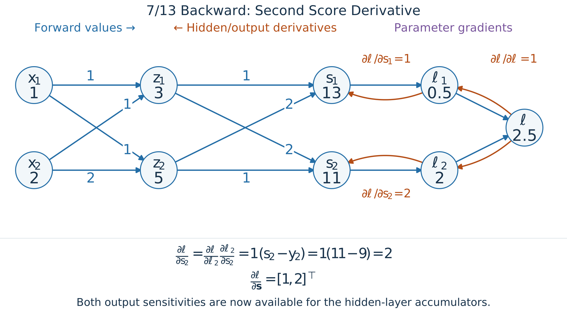
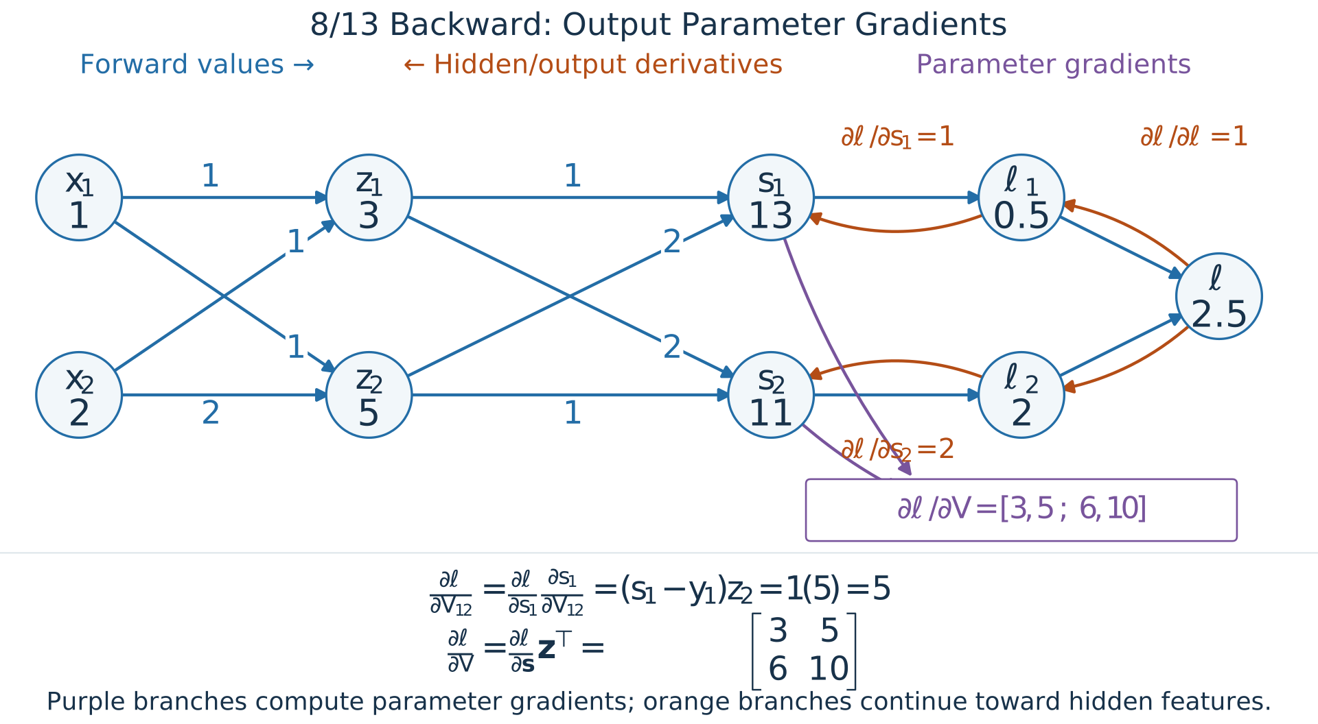
Training repeats forward, backward, and parameter updates

For a batch \(\mathcal B\) of \(B\) examples, use the mean loss:

\[J_{\mathcal B}(\boldsymbol\theta)=\frac1B\sum_{i\in\mathcal B}\ell_i(\boldsymbol\theta), \qquad \nabla_{\boldsymbol\theta}J_{\mathcal B}=\frac1B\sum_{i\in\mathcal B}\nabla_{\boldsymbol\theta}\ell_i.\]

1. Start: initialize the parameters once; choose a batch and clear old gradient accumulators.
2. Forward: compute predictions and the batch loss; save values needed for backward.
3. Backward: accumulate gradients for all trainable parameters, using the same parameter values.
4. Update: \(\boldsymbol\theta\leftarrow\boldsymbol\theta-\eta\nabla_{\boldsymbol\theta}J_{\mathcal B}\); repeat with a fresh forward pass.

An epoch visits the training set once. Monitor validation performance across epochs to choose when to stop.

About four minutes. This completes the algorithmic picture before the next topic implements it in PyTorch. The animation differentiates one example at fixed parameters; training averages such contributions across a batch before taking an update. Parameters are initialized once, not at each batch or epoch. Clear old batch gradients before the new independent accumulation; within the backward pass, sum every path contribution as illustrated by the hidden-feature accumulators. Apply the mean reduction exactly once. Batched operations need not materialize every example’s complete parameter gradient. Do not update a layer’s weights in the middle of the same backward pass. The shown update is SGD; the previously introduced Adam can use the same computed gradients. Recompute forward values after every update, and repeat batches over epochs. Validation guides settings and stopping; test data remain untouched. This is the unpenalized data objective; any explicit regularization term must also contribute its parameter derivatives. No PyTorch API is needed on this slide.

Libraries combine these rules to differentiate the whole network

1. Forward: record the operations and retain the values their backward rules need.
2. Backward: start at the scalar loss, apply local rules in reverse order, and sum contributions from shared paths.
3. Update: use the resulting gradient for every trainable parameter.

For an MLP with biases, that includes \(W,\boldsymbol b,V,\boldsymbol c\).

We specify the model and loss; automatic differentiation organizes the chain rule.

Next topic: implement this training cycle in PyTorch.

About two minutes. Do not turn this into a matrix-gradient derivation. Matrix multiplication, elementwise activations, softmax, and loss operations have local backward rules, just like the scalar atoms. Backpropagation is reverse-mode automatic differentiation applied to the network graph. The optimizer is a separate step. Gradients use the current parameters and saved forward values; repeated training steps require fresh forward computations. No framework-specific API or version claims are needed.

Backpropagation computes all parameter gradients efficiently

In 1D: \(\displaystyle\frac{\partial J}{\partial\theta}\approx\frac{J(\theta+\epsilon)-J(\theta)}{\epsilon}\).

One objective evaluation takes 1 second. Reuse the unperturbed value \(J(\boldsymbol\theta)\).

Finite differences: about how long for 10,000 parameters?

A. 2 seconds
B. 100 seconds
C. 10,000 seconds

C: 10,000 parameters → about 10,000 seconds.
One new evaluation per parameter.

Backpropagation: how long for the same full gradient?

Assume backward ≈ forward cost.

A. 2 seconds
B. 100 seconds
C. 10,000 seconds

A: about 2 seconds for forward + backward.
One reverse pass reuses work for all parameters.

About four minutes for two short votes and reveals. First show the 1D forward-difference formula; in many dimensions perturb one parameter at a time and hold the others fixed. Reusing one baseline evaluation gives P+1 evaluations in total, or P additional evaluations when the baseline is available: approximately 10,000 seconds for 10,000 parameters (about 2.8 hours). Use forward rather than central differences so the count matches the choices. Then reveal the second question and finally its answer. The illustrative two-second total assumes the backward pass costs about one forward pass; actual factors depend on operations and implementation. For standard differentiable scalar-loss computations, reverse-mode cost is a small multiple of forward cost, not an extra full evaluation per parameter. Forward cost itself may grow with model size; hold the stipulated one-second objective fixed for this comparison. Emphasize computational reuse, not approximation quality. Finite differences can still diagnose small gradient implementations, but are not the training method. Backpropagation computes gradients; an optimizer updates weights.