Convolutions and Image Structure
ECE 57000 — Fall 2026
Nearby pixels reveal local image patterns
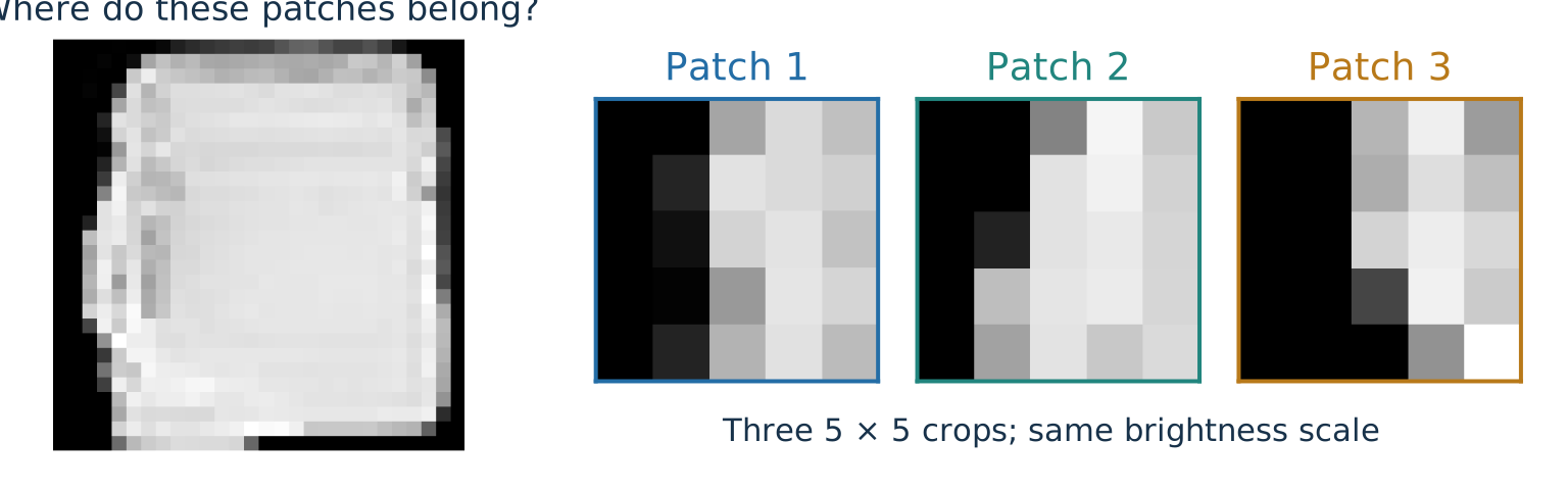
Where do these patches belong?
A. Left edge B. Interior C. Right edge
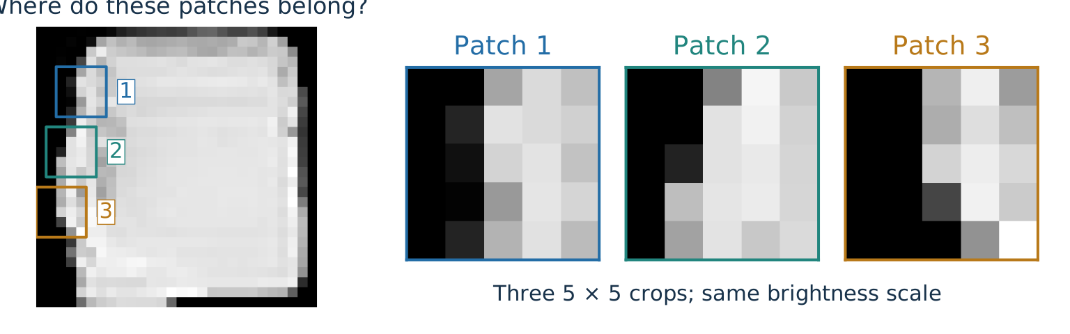
A. Left edge. Each patch goes from dark to bright. One local detector can find this pattern at many positions.
About three minutes including a short vote. First show the image and the three enlarged crops without source boxes. Ask where they could belong, rather than requiring an exact row match; similar local evidence does not uniquely specify position. Reveal the actual source boxes and their matching numbers together with the answer. These are three distinct 5-by-5 patches at separated heights on the same bag’s left boundary, using identical grayscale limits and no resizing before extraction. They are similar dark-to-light transitions, not identical patches. The bag is the first class-8 example in the existing training split. Crop rows are 4, 10, 16; each crop is centered near the first pixel exceeding 0.5 in its middle row. This deliberate illustrative selection is not an empirical accuracy experiment. Contrast the bright interior and opposite light-to-dark right edge. A local detector can respond wherever a similar pattern occurs; the next slides explain how shared weights implement such a rule. No claim that these hand-selected patches are learned filters. [Sources] source:fashion-mnist.
Image features have meaningful spatial neighbors
General feature vector: in [age, income, height], adjacent entries need not be more related than distant entries. Their order identifies features, not spatial neighbors.
Image: neighboring pixels measure nearby locations. Their arrangement forms edges, textures, and shapes.
Each hidden unit can use every pixel
Each output uses a local patch
Different units have independent weights
Reuse the same filter across locations
Can learn spatial relationships from data
Builds local reuse into the architecture
Convolution uses this structure: local neighborhoods matter, and a useful pattern may recur at different locations.
About three minutes. A vector is ordered: each feature must keep its identity consistently between training and use. However, arbitrary tabular column adjacency does not supply a spatial neighborhood. Permuting those columns consistently changes their indexing, not the underlying measurements. Image row/column positions have a spatial meaning; arbitrary pixel permutations disrupt local visual structure. Flattening with a known ordering is reversible and does not discard pixel values, but a fully connected layer does not explicitly exploit the original grid adjacency. Some vectors, such as time series, do have meaningful adjacency, so do not claim all vector data lack structure. An MLP can represent local rules, but the architecture does not enforce locality or tie corresponding weights. Convolution makes a particular prior convenient; fewer independent parameters do not guarantee better accuracy or fewer required examples in every task. This corrects the original deck’s overly broad translation-invariance claim: stride-one convolution is translation-equivariant away from boundary effects, not inherently an invariant classifier. [Sources] source:pytorch-conv2d-2-7.
Filters turn local patterns into computed features
Image structure · 2/3 Filters · Patterns → Filters → Networks
30-second transition. We identified a recurring local pattern. Now compute the same weighted rule at each location; then count its outputs and parameters.
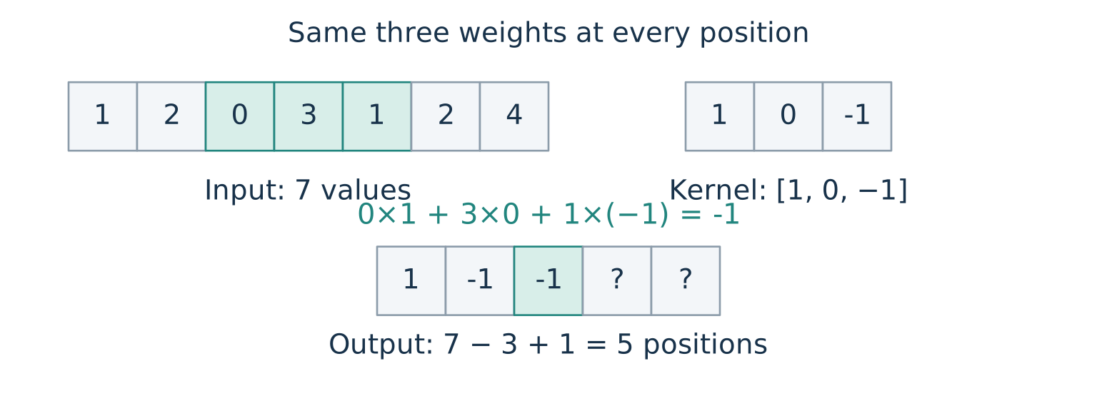
A convolution reuses one local weighted sum
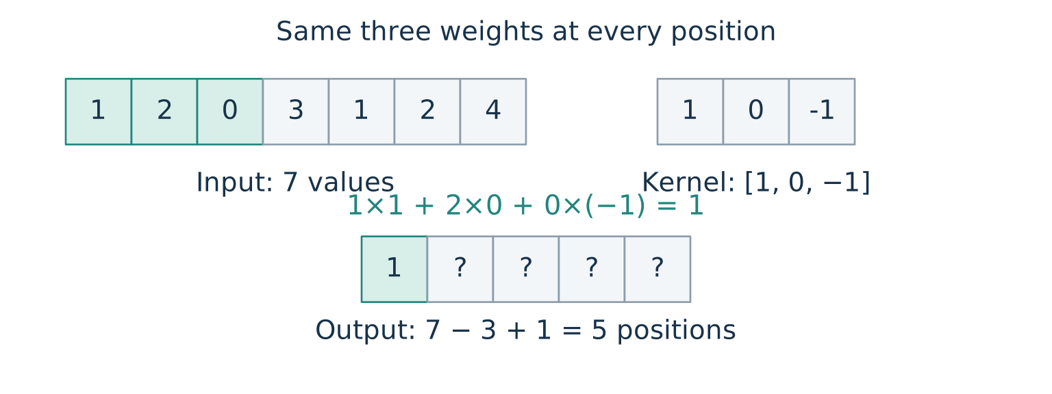
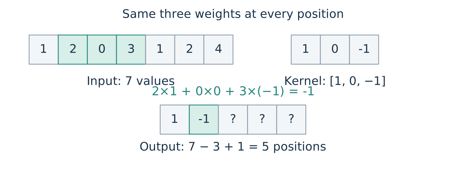
At each position: multiply the window entries by the same kernel entries, then add. A learned bias may be added to every result.
About three minutes. Advance through three positions: outputs 1, -1, -1; remaining outputs are 1 and -3. Kernel size three, stride one, no padding, and zero bias. Seven input entries admit five full windows. These illustrative weights are hand-set, whereas a learned layer trains them with backpropagation. PyTorch’s operation does not reverse the kernel: mathematically cross-correlation, conventionally called convolution in deep learning. [Sources] source:pytorch-conv2d-2-7.
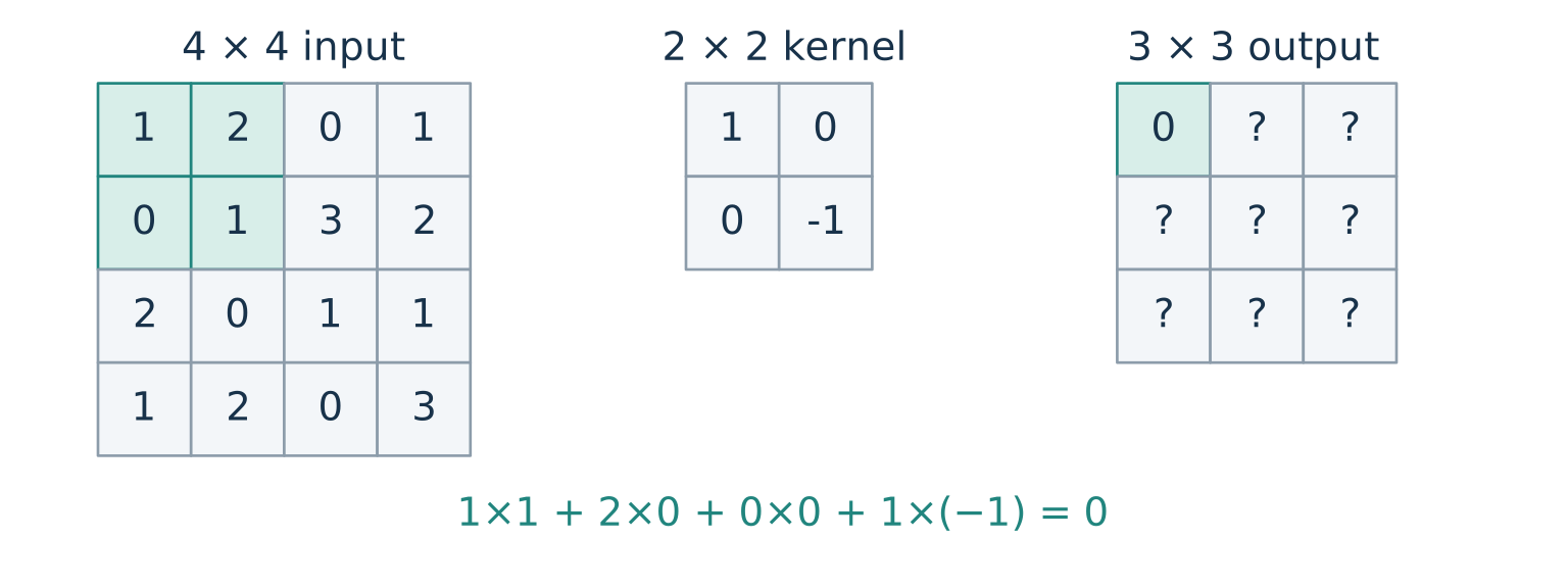
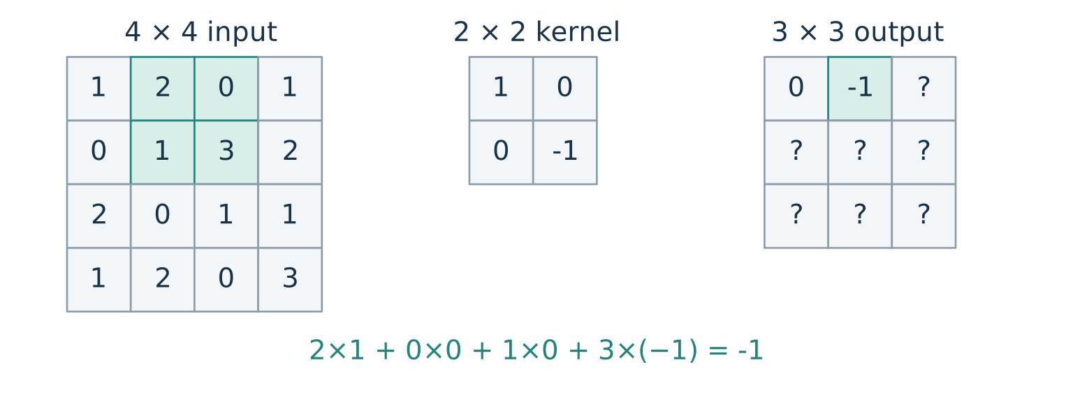
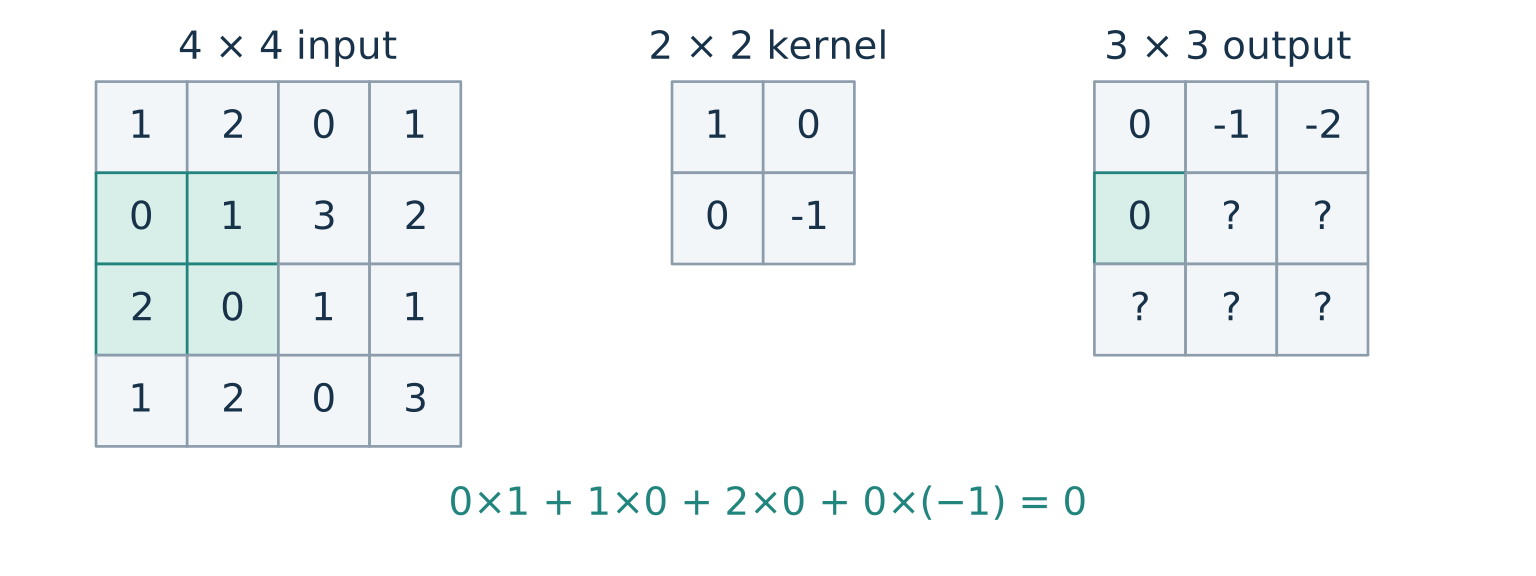
A 2D kernel slides across rows and columns
A \(2\times2\) window fits at three row starts and three column starts in a \(4\times4\) image: the output is \(3\times3\) .
About three minutes. Advance from the first position to the next column, then to the next row. The third frame includes the previously visited third entry of the first row. Use the shaded patch and output cell to connect each local weighted sum to one output position. Bias is zero here. No kernel reversal is used. An image with one channel is a matrix; channels are introduced after the spatial counting. [Sources] source:pytorch-conv2d-2-7.
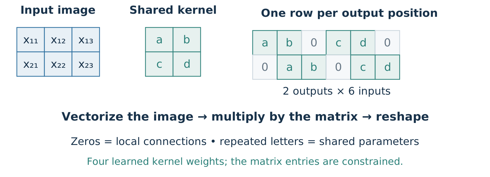
A convolution is a sparse matrix with shared entries
\[\operatorname{vec}(Y)=A_K\operatorname{vec}(X),\qquad A_K=\begin{bmatrix}a&b&0&c&d&0\\0&a&b&0&c&d\end{bmatrix}.\]
About three minutes. Formalize the explanation given orally on October 19. X is a 2×3 matrix, K is a 2×2 kernel, and Y is 1×2; vec stacks rows into a column here. Explicit row-major order: [x11,x12,x13,x21,x22,x23]^T. First row selects the left patch, second row the right patch. This uses PyTorch cross-correlation convention: no kernel flip. Four free weights, not twelve independent matrix parameters. A shared bias adds b_0 times the all-ones vector; omitted here to isolate the linear operator, with no activation. This is a conceptual matrix, not a recommendation to materialize it. Zeros express locality; tying expresses reuse. The numerical example X=[[1,2,3],[4,5,6]], K=[[1,2],[3,4]] gives [37,47]. Later reuse exactly this A_K to explain its transpose. [Sources] source:pytorch-conv2d-2-7.
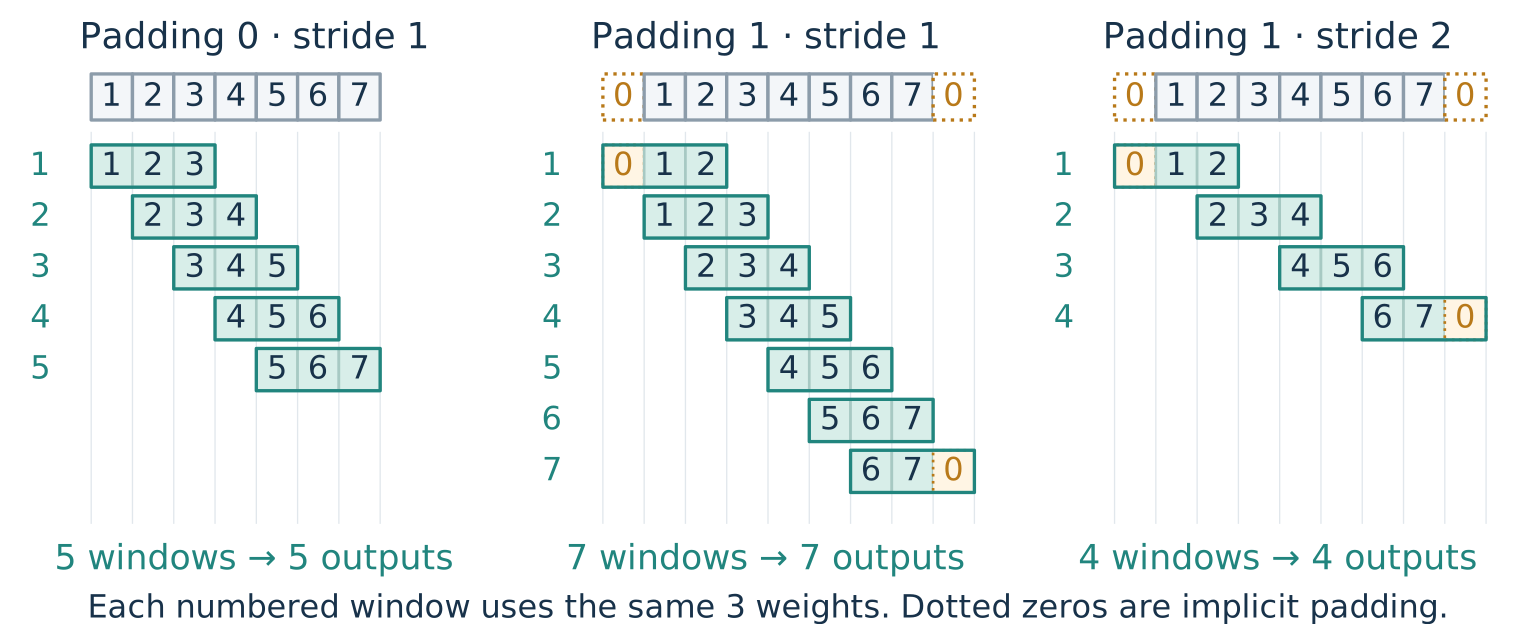
Padding adds a border; stride controls how quickly the window moves
Padding \(p\) : \(p\) implicit zeros on each side. Stride \(s\) : move \(s\) entries per step.
About three minutes. Compare the three panels on the same seven-value input and three-value kernel. Each numbered row shows one complete window aligned to the input above it; applying the same three weights produces one output. Without padding there are five windows. With one zero on both sides there are seven windows. Keeping that padding and moving two entries per step leaves four windows. Stride controls how quickly the window moves over the input, in entries per step, not computation time. The dotted zeros in the latter panels are outside the original input. Padding changes boundary information; zeros are an assumption, not observed pixels. Apply this independently to height and width. [Sources] source:pytorch-conv2d-2-7.
Spatial output size counts how many complete windows fit
Apply this separately to height and width . For either spatial dimension, use input size \(n\) , kernel size \(k\) , padding \(p\) , and stride \(s\) :
\[n_{\mathrm{out}}=\left\lfloor\frac{n+2p-k}{s}\right\rfloor+1.\]
\(n+2p-k\) : distance from the first valid start to the last possible start.Divide by \(s\) and round down: number of full moves.
Add one: include the first window.
Example: \(n=7,\ k=3,\ p=1,\ s=2\) gives \(\lfloor(7+2-3)/2\rfloor+1=4\) .
Next: channels. Their output count follows a different rule.
About three minutes. Apply the same formula separately to height and width, allowing different settings on the two axes. All examples in this topic use dilation one, symmetric zero padding, and groups one. If dilation is introduced later, the effective kernel size is d(k-1)+1. If the padded input is smaller than the kernel there is no valid output, and PyTorch rejects that configuration. [Sources] source:pytorch-conv2d-2-7.
Multiple filters create multiple output channels
One filter → one output channel; \(c_{\mathrm{out}}\) filters → \(c_{\mathrm{out}}\) output channels.
\[[B,c_{\mathrm{in}},h,w]\quad\longrightarrow\quad[B,c_{\mathrm{out}},h_{\mathrm{out}},w_{\mathrm{out}}].\]
Batch size \(B\)
Unchanged: apply the same filters to each example
Output channels \(c_{\mathrm{out}}\)
Number of learned filters we choose
Height and width
Kernel size, padding, and stride
nn.Conv2d(3, 16, kernel_size=5, padding=2) maps [64, 3, 28, 28] → [64, 16, 28, 28] .
The weight tensor has shape [16, 3, 5, 5] : sixteen filters, each spanning three input channels.
About three minutes. Declare B as the conventional batch-axis label, and lowercase c,h,w as scalar sizes. Array shapes are ordered axis lengths, not vector values. PyTorch uses batch, channel, height, width. Output channels are an architectural choice, independent of the spatial size calculation. Continue the preceding 5-by-5 filter example. Padding two preserves spatial size; stride defaults to one. [Sources] source:pytorch-conv2d-2-7.
Parameter reuse is a core neural-network design principleSame input/output: \(c\times h\times w\) ; counts below use \(1\times28\times28\)
MAC = multiply–accumulate; excludes bias additions. Kernels are \(k\times k\) , stride 1.
Fully connected
615,440
614,656
\(O(c^2h^2w^2)\) \(O(c^2h^2w^2)\)
Conv \(3\times3\) , padding 1
10
7,056
\(O(k^2c^2)\) \(O(k^2c^2hw)\)
Conv \(5\times5\) , padding 2
26
19,600
\(O(k^2c^2)\) \(O(k^2c^2hw)\)
Parameters = weights + biases: convolution \(k^2c^2+c\) ; fully connected \((chw)^2+chw\) .
Efficiency: local connections reduce computation; shared weights reduce parameter memory.Generalization: reuse can help when the same patterns recur across positions.Looking ahead: transformers also reuse parameters across positions.
About four minutes. Compare a flattened fully connected layer from chw inputs to chw outputs with an ordinary dense convolution from c input channels to c output channels, reshaping the fully connected output to the same spatial shape. The concrete example is grayscale, c=1, h=w=28. Fully connected weights and MACs are (chw)^2; convolution weights are k^2 c^2 and MACs are hw k^2 c^2. Thus 784^2=614656, 9×784=7056, and 25×784=19600 MACs. Parameter totals include biases: fully connected has (chw)^2+chw=615440, and convolution has k^2 c^2+c, giving 10 or 26. Biases add chw additions per image in either case, excluded from MAC counts. These lower-order bias terms do not change the displayed big-O scaling. Padding (k-1)/2 and stride one preserve spatial size. MACs use the standard dense-kernel count including padded positions; implementations can skip work or use other algorithms, so these counts are not wall-clock timing predictions. Each MAC is approximately two floating-point operations. Keep kernel size explicit as O(k^2 c^2) parameters and O(k^2 c^2 hw) MACs in the table; substitute k=3 or k=5 for the numerical examples. Distinguish local connectivity from sharing: an unshared local layer would perform the same local weighted sums but require separate weights at every position. Parameter reuse saves storage and ties statistical estimates across positions; it does not by itself eliminate those weighted sums. Reuse can improve generalization when the repeated-pattern assumption is appropriate, but may hurt when position-specific patterns matter. Transformer token projections and feed-forward layers will reuse weights across token positions; this does not imply their attention computation has CNN complexity. [Sources] source:pytorch-conv2d-2-7.
Networks connect filters through compatible shapes
Image structure · 3/3 Networks · Patterns → Filters → Networks
30-second transition. Local filtering established the operation and its parameter sharing. Now choose spatial sizes and channel counts so successive layers fit together.
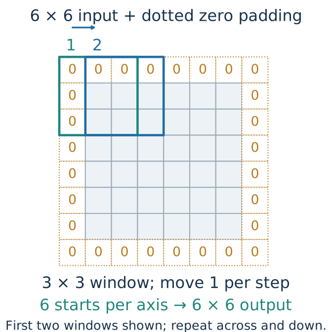
Odd kernels with matching padding preserve spatial size
With stride 1, choose \(p=(k-1)/2\) for odd \(k\) .
\(1\times1\) 0
\(28-1+1=28\)
\(3\times3\) 1
\(28+2-3+1=28\)
\(5\times5\) 2
\(28+4-5+1=28\)
Apply to height and width: \(28\times28\to28\times28\)
Same spatial size does not mean same channel count. We choose the number of filters.
About three minutes. The diagram uses a smaller 6-by-6 input for readability; the same rule gives 28-by-28 output for the table. Green and blue outlines show the first two windows. Repeat the movement across and down. These are the three size-preserving cases in the instructor’s original CNN slides. Padding is per side, so padding two adds four entries per axis. We specify numerical padding instead of relying on a library’s same-padding keyword. All examples use dilation one. [Sources] source:pytorch-conv2d-2-7.
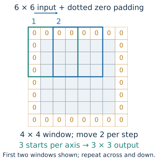
Stride two can halve each spatial dimension
With stride 2 , count starts along each axis:
\(2\times2\) 0
\(\lfloor(28-2)/2\rfloor+1=14\)
\(4\times4\) 1
\(\lfloor(28+2-4)/2\rfloor+1=14\)
\(3\times3\) 1
\(\lfloor(28+2-3)/2\rfloor+1=14\)
\(28\times28\to14\times14\) :
Check odd sizes: from 27, the first two cases produce 13; the third produces 14.
About three minutes. The diagram uses a 6-by-6 input, padding one, and a 4-by-4 kernel. The first two windows start two entries apart. Starts 0, 2, and 4 along each padded axis give 3-by-3 output. At size 28, the same rule gives 14-by-14. The first two settings are exactly the downsampling examples from the original slides; the third is the common setting used in our small CNN. Have students compute the numerator and floor before adding one. Do not promise exact halving for odd sizes. Striding can lose fine spatial information; later shape equality does not recover discarded information. [Sources] source:pytorch-conv2d-2-7.
A \(1\times1\) convolution mixes channels at each location
At each pixel location, apply the same linear layer to its vector of channel values.
\[[B,16,28,28]\quad\xrightarrow{\ 1\times1,\ s=1,\ p=0\ }\quad[B,8,28,28].\]
No neighboring pixels are combined.
Sixteen input channels become eight learned output features at each location.
Parameter count with bias: \(8(16+1)=136\) .
A one-pixel kernel can still learn a useful transformation.
About two minutes. This case counters the idea that kernel size one must be an identity. A linear map mixes channels at each position; bias makes it technically affine. With just one input and output channel it is a shared scalar rescaling and bias, still not necessarily identity. [Sources] source:pytorch-conv2d-2-7.
Stacking local layers combines increasingly broad patterns
Two \(3\times3\) convolutions with stride 1 let an interior output depend on a \(5\times5\) input region
\[1\times1\ \xrightarrow{\text{first }3\times3}\ 3\times3\ \xrightarrow{\text{second }3\times3}\ 5\times5.\]
This dependency region is the receptive field . Each new local window combines neighboring features from the previous layer.
Insert ReLU between layers to learn nonlinear combinations of those features.
About two minutes. Read the expression as growth in the input dependency region, not feature-map shapes: with padding one the feature maps can remain 28 by 28 throughout. Each stride-one size-three layer extends the radius by one pixel. This is the theoretical receptive field; learned weights and activation states determine the actual influence. Without intervening nonlinearities a composition remains a linear map, up to biases. Boundary padding changes which dependencies refer to observed pixels.
A small CNN changes the model but reuses the training loop
= nn.Sequential(1 , 8 , 3 , padding= 1 ),8 , 16 , 3 , stride= 2 , padding= 1 ),16 * 14 * 14 , 10 ))= torch.zeros(64 , 1 , 28 , 28 )for layer in cnn:= layer(a)print (type (layer).__name__ , tuple (a.shape))Output:
About four minutes. Every line of output is captured from the verified model in arc5_convolution_figures.py. Zero inputs are only a shape probe, not training data. ReLU preserves shape, Flatten keeps the batch axis, and the final layer supplies ten logits for the same cross-entropy. To train this new model, construct its optimizer from cnn.parameters(), then pass cnn and that optimizer to the existing train_one_epoch and evaluate helpers. Do not reuse the old MLP’s optimizer. This model has 32,618 parameters; the next topic reports its fixed-protocol comparison. [Sources] source:pytorch-conv2d-2-7.
Keep the pixels, change their arrangement
Randomly permute pixel positions. Use the same permutation for every image , then retrain both models.
Which model’s architectural advantage would you expect to shrink?
A. MLP
B. CNN
C. Both equally
B. CNN. The information remains, but nearby entries no longer form local image patterns.
About three minutes including voting. Central emphasis: architecture helps by matching structure in the data, not by creating additional input information. This question follows the complete CNN and leads directly into evaluating its assumptions. B is the best prediction about the locality/shared-pattern advantage, not a guaranteed accuracy ranking. C is tempting because the shuffled image looks equally scrambled to a person; A may reflect the idea that an MLP cannot undo a shuffle. A fixed permutation loses no pixel information, and a fully connected first layer can absorb it by permuting its input weights. In contrast, convolution now ties local rules over arbitrary neighborhoods rather than nearby image locations. This does not prove every CNN must perform worse or that finite training gives exactly the same MLP accuracy. A different random permutation for each image would be a different experiment. We have not measured this intervention; the next section measures the original models and a separately defined translation stress. Do not turn this into a detour on permutation notation.
Convolution provides structure, not a guarantee of accuracy
Locality: each output sees a patch, expanded by stacking layers.Sharing: the same filters are reused across positions.Shape control: filters choose channels; kernel, padding, and stride choose spatial sizes.
Next, compare CNN and MLP using the same data splits and a documented training/selection protocol.
The design is now explicit. Its benefit is an empirical question.
About one minute. Wrap the operation and shape intuitions before empirical architecture evaluation. Save the position/invariance distinction for the prediction question and counterexample in the next topic; do not preempt its reveal. The next topic measures these particular models under a fixed classroom protocol; do not generalize its result to every CNN. [Sources] source:pytorch-conv2d-2-7.