Dimensionality Reduction and Linear Transformations

ECE 57000 — September 4, 2026

David I. Inouye

Wednesday established why dimensionality reduction is needed

We began with data that computers can process but people cannot inspect directly:

\(500\) cells \(\times\) \(20{,}000\) measurements per cell

Goal 1: visualization

Reveal clusters, unusual points, and other hidden structure.

Goal 2: further analysis

Use fewer features for cheaper computation and potentially more reliable statistical estimation.

The unresolved question is what useful structure the reduced representation should retain.

Keep this recap brief. The September 2 frozen snapshot ended on “Both goals lead to the problem of dimensionality reduction.” Resume by recalling the motivating dataset, the two goals, and the unresolved preservation question; then move directly into visual examples of structural tradeoffs.

What kind of structure do we want to maintain?

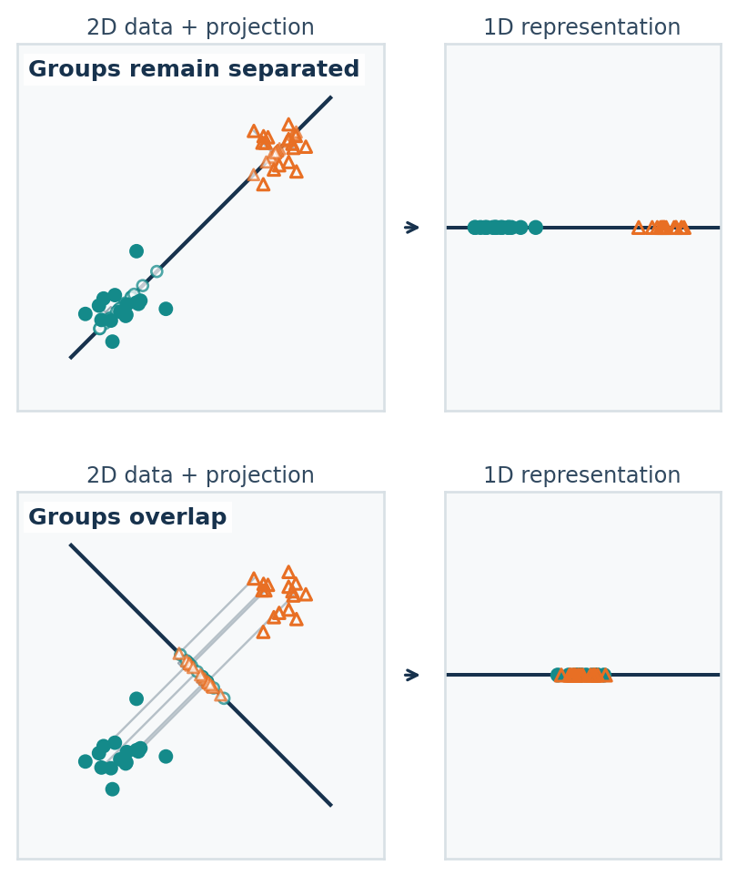
Groups and neighborhoods. Keep nearby points close and distinct groups separate when those relationships matter.

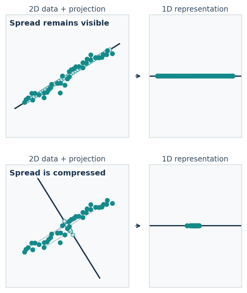
Spread. Retain directions in which the observations vary rather than compressing meaningful variation.

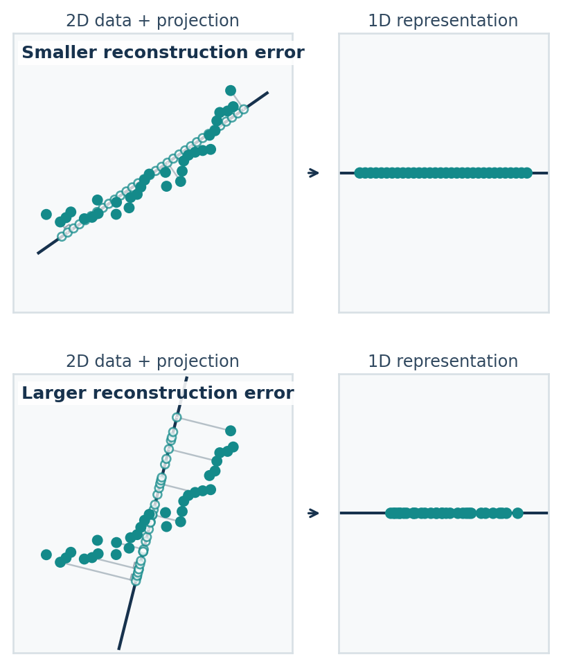
Reconstruction. Prefer features that can recover points close to their original 2D locations when reconstruction matters.

How do we formalize these criteria?

We need the language of vectors, geometry, and linear transformations.

Read each column from top to bottom. The data do not change; only the chosen projection direction changes. Light perpendicular segments show selected points being projected onto the line, and the right-hand box shows the resulting 1D feature values. Open triangles distinguish the orange group when its feature values overlap the teal group.

Keep this discussion visual. After students have norms, projections, and variance, return to these same structures and formalize them as distances, neighborhood relations, retained spread, and reconstruction error. The reconstruction example uses exactly the same slightly curved, noisy observations in both rows; the line, not the dataset, changes. Do not introduce the zero-scaling or exact-recoverability distinction here.

Formalization starts by naming one observation

For cell \(i\), collect its \(d\) measured features into a vector:

\[ \boldsymbol{x}_i = \begin{bmatrix} x_{i1} & x_{i2} & \cdots & x_{id} \end{bmatrix}^{T} \in \mathbb{R}^{d} \]

• \(i\) identifies the cell.
• \(j\) identifies a measured feature such as one gene.
• \(d\) is the number of observed features—not automatically the number of meaningful directions in the data.

A data matrix records features—not intrinsic dimension

Stack \(n\) observations as rows:

\[ X = \begin{bmatrix} ---\boldsymbol{x}_1^T---\\ ---\boldsymbol{x}_2^T---\\ \vdots\\ ---\boldsymbol{x}_n^T--- \end{bmatrix} \in \mathbb{R}^{n\times d} \]

rows \(=\) observations
columns \(=\) measured features

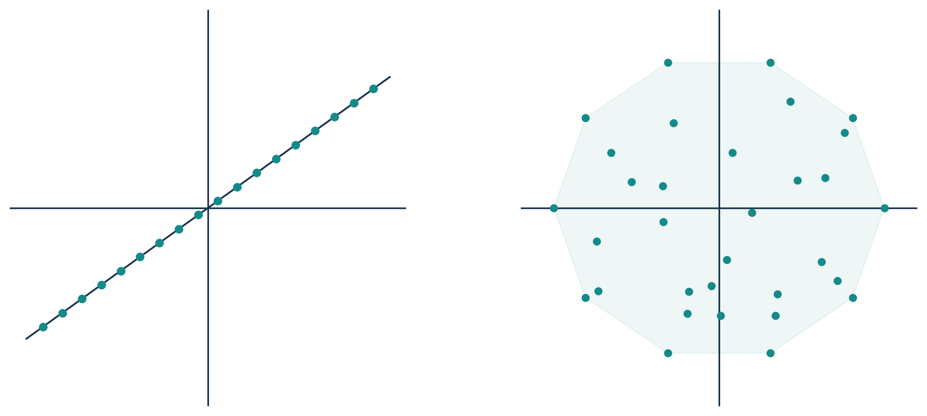
1D structure in 2D

2D structure in 2D

Both datasets have two measured features; only one needs two independent directions to describe its variation.

Connect matrix shape to ambient dimension without equating it with the dimension of the observed structure. The left dataset has two feature columns but varies along one line. The right varies across an area and requires two independent directions. This is an intuition for intrinsic dimension; no rank calculation is needed yet.

We seek a function from observed to reduced features

For each observation, seek

\[ f:\mathbb{R}^{d}\rightarrow\mathbb{R}^{k}, \qquad \boldsymbol{z}_i=f(\boldsymbol{x}_i), \qquad k\ll d, \]

where \(\boldsymbol{x}_i\in\mathcal{X}\subseteq\mathbb{R}^{d}\) contains the observed features and \(\boldsymbol{z}_i\in\mathcal{Z}\subseteq\mathbb{R}^{k}\) contains the reduced features.

For now, assume \(f\) is linear. Later, we will learn nonlinear representation functions—but linear transformations are the foundation for analyzing both.

To define, analyze, and choose this \(f\), we need linear algebra for geometry, transformations, and lower-dimensional structure.

The function notation is formal and sufficient here: it states the domain, codomain, and how one observation is transformed. Do not pause to teach arrow notation. Emphasize that linear algebra is the language needed to formalize and analyze this problem, and a foundation for later nonlinear models. Briefly name geometry, transformations, and lower-dimensional structure; the next topic will unpack them through norms, orthogonality, rank, projection, and decompositions.

The problem organizes what comes next

We began with a need: make high-dimensional relationships inspectable without pretending every relationship survives.

We now have:

1. an explicit purpose and candidate preservation criteria;
2. observations \(\boldsymbol{x}_i\), a data matrix \(X\), and desired reduced features \(Z\);
3. a visual distinction among neighborhoods, spread, and reconstruction; and
4. a concrete reason to develop the linear algebra needed to finish the model.

Linear Transformations: What Do They Do?

This topic treats a matrix as a transformation between feature spaces. Keep the 1D scalar analogy visible throughout. SVD ends the topic as an explanatory fact; rank, projection, inversion, and PCA follow in the next topic.

A linear representation turns the problem into a matrix question

We began with a representation function:

\[ f:\mathbb{R}^{d}\rightarrow\mathbb{R}^{m}, \qquad \boldsymbol{y}=f(\boldsymbol{x}). \]

For this first representation model, assume \(f\) is linear:

\[ \boldsymbol{y}=A\boldsymbol{x}, \qquad A\in\mathbb{R}^{m\times d}. \]

What can this transformation do to a high-dimensional feature space?

Reconnect to the previous topic without repeating its full setup. The symbols change from reduced features z to generic output features y because this topic studies any linear transformation, including ones that increase dimension.

Matrix multiplication generalizes scalar multiplication

One dimension

\[ y=ax \]

• \(x,y,a\) are scalars.
• \(a\) scales one number line.
• The sign can reverse direction.

Higher dimensions

\[ \boldsymbol{y}=A\boldsymbol{x} \]

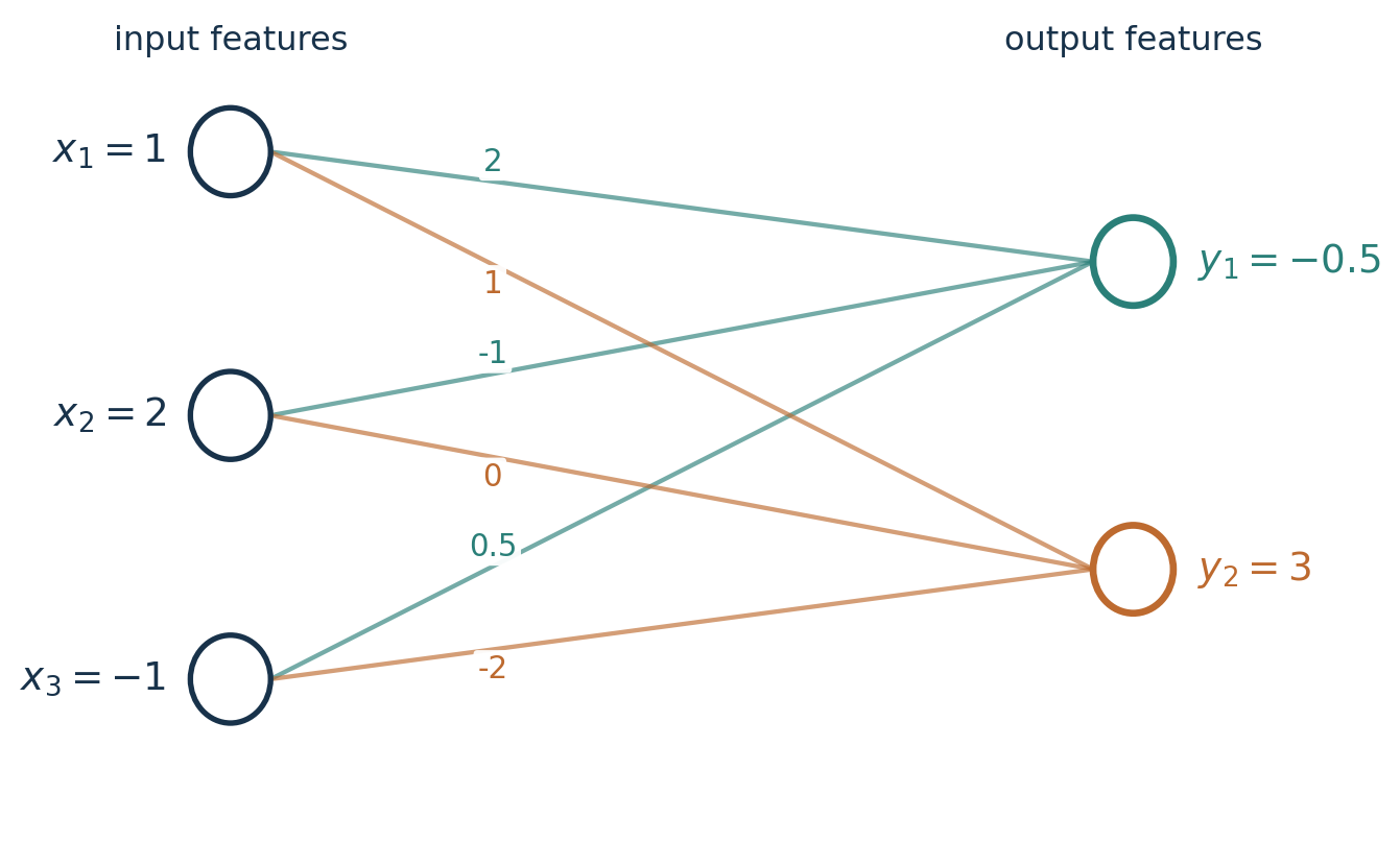
• \(\boldsymbol{x}\) and \(\boldsymbol{y}\) are vectors.
• \(A\) can scale different directions differently.
• Input and output can have different dimensions.

\(a\) becomes \(A\): one scalar action becomes a transformation of a feature space.

Use this correspondence repeatedly. Do not imply that A merely scales the coordinate axes as written; the later SVD shows the directions in which the independent scalar actions occur.

Each output feature receives a weighted connection from every input

\[ A= \begin{bmatrix} 2 & -1 & 0.5\\ 1 & 0 & -2 \end{bmatrix} \]

• A teal edge contributes to \(y_1\).
• An orange edge contributes to \(y_2\).
• Every edge weight is one entry \(a_{ji}\).

Trace one input value along both outgoing edges. The diagram resembles a neural network, but do not introduce that term yet. Its purpose is to make an ordinary matrix multiplication visible as weighted connections.

Every output is a different linear combination of the inputs

\[ \begin{aligned} y_1 &=2x_1-x_2+0.5x_3\\ &=2(1)-2+0.5(-1)\\ &=-0.5 \end{aligned} \]

\[ \begin{aligned} y_2 &=x_1+0x_2-2x_3\\ &=1+0-2(-1)\\ &=3 \end{aligned} \]

\[ \underbrace{ \begin{bmatrix}-0.5\\3\end{bmatrix} }_{\boldsymbol{y}} = \underbrace{ \begin{bmatrix}2&-1&0.5\\1&0&-2\end{bmatrix} }_{A} \underbrace{ \begin{bmatrix}1\\2\\-1\end{bmatrix} }_{\boldsymbol{x}} \]

First read each scalar equation. On reveal, align each equation with one row of A. Row-by-column multiplication is the mechanism; the weighted combination is its meaning.

One matrix applies the same transformation to every observation

For observation \(i\):

\[ \boldsymbol{y}_i=A\boldsymbol{x}_i, \qquad \boldsymbol{x}_i\in\mathbb{R}^{d}, \quad \boldsymbol{y}_i\in\mathbb{R}^{m}. \]

The same entries of \(A\) define every output feature for every observation.

• Convention: Vectors such as \(\boldsymbol{x}_i\) are usually written as columns.
• Transpose: \(A^T\) swaps rows and columns: \(A\in\mathbb{R}^{m\times d}\Rightarrow A^T\in\mathbb{R}^{d\times m}\).

One linear operator gives a consistent representation rule for the entire dataset.

Prepare the batch activity without yet displaying its answer. Emphasize that A contains parameters of the representation, while each observation supplies new input values.

Which batch equation has the right shape?

Observations are rows:

\[ X=\begin{bmatrix} 1&2&-1\\ 0&1&2\\ 2&-1&1 \end{bmatrix} \]

Use the same transformation:

\[ A=\begin{bmatrix} 2&-1&0.5\\ 1&0&-2 \end{bmatrix} \]

Compute \(Y\) with one matrix multiplication

\[Y=\text{???}\]

\[ \underbrace{Y}_{3\times2} =\underbrace{X}_{3\times3}\underbrace{A^T}_{3\times2} =\begin{bmatrix} -0.5&3\\ 0&-4\\ 5.5&0 \end{bmatrix} \]

Each row of \(Y\) is \((A\boldsymbol{x}_i)^T\).

Activity, about 2 minutes. Ask students to construct the batch equation and predict its shape before revealing the answer. A strong response checks the inner dimensions and reconciles column-vector mathematics with row-stacked data.

Matrix algebra preserves some scalar rules and rejects others

Valid for scalars and matrices

\[ A(B\boldsymbol{x})=(AB)\boldsymbol{x} \]

\[ A(\boldsymbol{x}+\boldsymbol{z}) =A\boldsymbol{x}+A\boldsymbol{z} \]

\[ AI=A \]

Order matters for matrices

\[ AB\ne BA \quad \text{in general} \]

\[ (AB)^T=B^TA^T \]

Changing the order can change the value or make the product undefined.

Students do not need the property names as vocabulary targets. They do need to know which rearrangements preserve an equation. Contrast scalar commutativity with matrix order and point out that dimensions often expose an invalid move.

Dimensions expose many invalid manipulations

Let \(A\in\mathbb{R}^{m\times d}\) and \(B\in\mathbb{R}^{d\times p}\).

Valid

\[ AB\in\mathbb{R}^{m\times p} \]

\[ (AB)^T=B^TA^T \]

Not guaranteed to exist

\[ BA \]

The inner dimensions would require \(p=m\).

Shape is part of the mathematical claim, not an implementation detail.

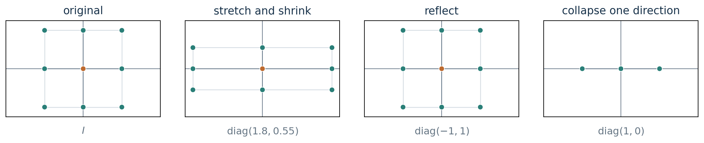
A diagonal matrix applies a separate 1D scaling to each feature

A zero diagonal entry behaves like \(a=0\): one direction becomes a partial zero.

Connect each diagonal entry to an independent scalar multiplier. The final panel previews singularity without generalizing it yet: after SVD, any matrix with a zero singular value will contain this same irreversible action in some direction.

The Euclidean norm measures size and distance

For \(\boldsymbol{x}\in\mathbb{R}^{d}\):

\[ \lVert\boldsymbol{x}\rVert_2 =\sqrt{x_1^2+x_2^2+\cdots+x_d^2} \]

For two points \(\boldsymbol{x}_i\) and \(\boldsymbol{x}_j\):

\[ \operatorname{dist}(\boldsymbol{x}_i,\boldsymbol{x}_j) =\lVert\boldsymbol{x}_i-\boldsymbol{x}_j\rVert_2 \]

The subscript \(2\) identifies the Euclidean norm. Other norms measure size differently.

This is the only norm needed now. Keep L1 and infinity norms for later problems where their different geometry or robustness matters.