Linear Transformations: What Do They Do? (continued)

ECE 57000 — September 9, 2026

David I. Inouye

Milestone 1: let stakeholder needs shape your idea

The goal is a credible match between a stakeholder’s needs and something you can provide.

Two Starting Paths

• Stakeholder first (recommended): identify people, research their work, then explore their needs.
• Idea first (also okay): bring a tentative idea to relevant people and let their priorities reshape it.

Your idea is a starting hypothesis. Seek a problem they care about solving.

Reach Out Early

1. Learn enough about their context to ask useful questions.
2. Invite a brief email exchange or call, if they are interested.
3. Ask about needs, pain points, and what would help.
4. Offer a few concise ideas as conversation starters; refine them together as you learn.

Instructor guidance for the existing Milestone 1 product value case, not a new submission requirement. Encourage students to listen before pitching. Starting with an idea is acceptable; finding someone who politely likes it is weak evidence of value. Respect whether the person wants to engage. Emphasize that helping the stakeholder is the goal and that early suggestions are provisional.

Design thinking makes learning from people part of the process

Mode	What You Do
Empathize	Learn about people’s work, experiences, and priorities.
Define	Frame a specific need in its real context.
Ideate	Explore several ways to address that need.
Prototype	Make a small, inexpensive version people can react to.
Test	Observe what helps; revise the idea or the problem definition.

Return to earlier modes as you learn. Stakeholders help shape both the problem and the solution.

[Sources] source:stanford-design-thinking-bootleg-2018 Overview modes, PDF pages 3–12. These are iterative modes, not a mandatory five-stage checklist. For Milestone 1, emphasize understanding and framing the need, while keeping solution ideas tentative. A prototype may be a sketch or acted-out workflow; students do not need to build software to start learning.

Process adapted from Stanford d.school’s Design Thinking Bootleg (PDF) (website).

A useful first conversation explores their actual experience

Suggested Quickstart

• Prepare around a stakeholder’s context; invite a short conversation.
• Ask: “Can you walk me through the last time this was difficult?”
• Follow up: “How do you handle it today? What would make a meaningful difference?”
• Summarize what you heard, check your interpretation, then explore possible help.

Optional Starting Resources

• Practical tools: Design Thinking Bootleg cards (PDF) (website) — begin with Interview Preparation and Interview for Empathy (cards 3–4).
• Another process map: Design Council’s Double Diamond — Discover → Define → Develop → Deliver; explore and narrow both the problem and possible solutions.

[Sources] source:stanford-design-thinking-bootleg-2018 [Sources] source:design-council-framework-for-innovation Suggested questions are instructor-authored examples informed by the Bootleg’s interview methods, not quotations. Ask about specific past situations and current workarounds; avoid leading the conversation toward praise for your proposed app. Separate what was said from your interpretation and check back with the person. These are optional resources, not additional reading or interview requirements. The Double Diamond is a related framework, not an unrelated competing theory.

Friday connected dimensionality reduction to linear transformations

Formalize the representation

• One observation: \(\boldsymbol{x}_i\in\mathbb{R}^{d}\)
• Reduced features: \(\boldsymbol{z}_i=f(\boldsymbol{x}_i)\in\mathbb{R}^{k}\)
• First foundational case: \(f\) is linear

Reason through the operator

• \(\boldsymbol{y}=A\boldsymbol{x}\): each output is a linear combination
• \(Y=XA^T\): one operator transforms every observation
• Shapes expose invalid matrix manipulations

Diagonal matrices scale features independently; the Euclidean norm formalizes vector size and pairwise distance.

Keep this recap concise. Friday completed the dimensionality-reduction problem setup, developed matrix multiplication and batch notation, and ended on the Euclidean norm. Repeat that final slide next for continuity, then use distance to motivate orthogonality.

The Euclidean norm measures size and distance

For \(\boldsymbol{x}\in\mathbb{R}^{d}\):

\[ \lVert\boldsymbol{x}\rVert_2 =\sqrt{x_1^2+x_2^2+\cdots+x_d^2} \]

For two points \(\boldsymbol{x}_i\) and \(\boldsymbol{x}_j\):

\[ \operatorname{dist}(\boldsymbol{x}_i,\boldsymbol{x}_j) =\lVert\boldsymbol{x}_i-\boldsymbol{x}_j\rVert_2 \]

The subscript \(2\) identifies the Euclidean norm. Other norms measure size differently.

This is the only norm needed now. Keep L1 and infinity norms for later problems where their different geometry or robustness matters.

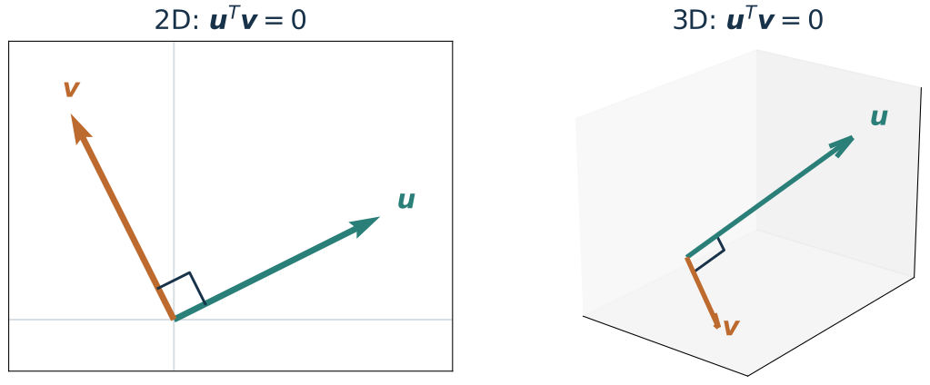
Orthogonal vectors meet at a right angle

\[ \boldsymbol{u}\perp\boldsymbol{v} \quad\Longleftrightarrow\quad \boldsymbol{u}^{T}\boldsymbol{v}=0 \]

Define the perpendicular symbol before using it. In two and three dimensions, students can see a right angle. The zero inner product is the definition that continues to work when a picture is impossible.

In higher dimensions, we compute orthogonality

Are these dense five-dimensional vectors orthogonal?

\[ \boldsymbol{u}=\begin{bmatrix}1\\2\\-1\\3\\4\end{bmatrix}, \qquad \boldsymbol{v}=\begin{bmatrix}2\\-1\\3\\2\\-\tfrac34\end{bmatrix} \]

\[ \boldsymbol{u}^{T}\boldsymbol{v} =2-2-3+6-3 =0 \qquad\Longrightarrow\qquad \boldsymbol{u}\perp\boldsymbol{v} \]

Orthogonality is defined in any dimension, even when geometry cannot be visualized.

Pause before revealing the dot product. Every coordinate is nonzero, and no visual inspection makes the relationship obvious. This is why the algebraic definition matters in high-dimensional spaces.

An orthogonal matrix has orthonormal columns

For a square matrix \(Q=[\boldsymbol{q}_1\;\cdots\;\boldsymbol{q}_d]\in\mathbb{R}^{d\times d}\), orthonormal means mutually orthogonal columns, each of unit length.

Higher dimensions	Interpretation	1D special case	Interpretation
\(I\boldsymbol{x}=\boldsymbol{x}\)	The identity matrix leaves a vector unchanged.	\(1x=x\)	The scalar \(1\) leaves a number unchanged.
\((Q^TQ)_{ij}=\boldsymbol{q}_i^T\boldsymbol{q}_j\)	Multiplication collects all column inner products.	\(q\,q=q^2\)	There is only one entry to multiply by itself.
\(Q^TQ=I\)	Inner products are \(1\) for the same column, \(0\) for distinct columns.	\(q^2=1\)	Hence \(q\in\{-1,1\}\).
\(\boldsymbol{y}=Q\boldsymbol{x}\)	Rotates or reflects about the origin, preserving length.	\(y=qx\)	Keeps or reverses direction while preserving length.

Introduce the higher-dimensional definition first, then read each row from left to right to connect it to the 1D special case Q = [q]. The identity matrix plays exactly the role of 1. Q transpose Q is the table of column inner products: the diagonal entries are squared column lengths, and off-diagonal entries test orthogonality. In 1D, transpose changes nothing and the condition reduces to q squared equals one. The final row previews the geometric interpretation; the next two slides ask students to predict distance preservation and prove it.

Do orthogonal transformations preserve every pairwise distance?

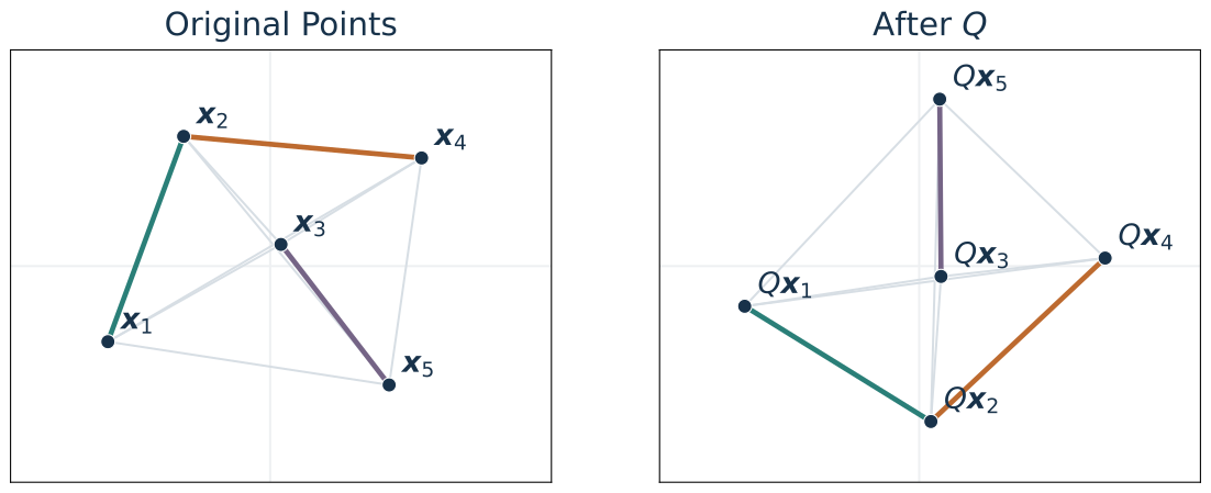
Is \(\lVert Q\boldsymbol{x}_i-Q\boldsymbol{x}_j\rVert_2\) equal to \(\lVert\boldsymbol{x}_i-\boldsymbol{x}_j\rVert_2\) for every pair?

Pause for a prediction. The entire configuration appears rotated and reflected; the highlighted segments make several pairwise comparisons visible without claiming that only those pairs are preserved.

Orthogonality preserves all pairwise Euclidean distances

For any \(\boldsymbol{x}_i,\boldsymbol{x}_j\in\mathbb{R}^{d}\) and orthogonal \(Q\):

\(\displaystyle \lVert Q\boldsymbol{x}_i-Q\boldsymbol{x}_j\rVert_2\)

\(=\)

\(\displaystyle \lVert Q(\boldsymbol{x}_i-\boldsymbol{x}_j)\rVert_2\)

(Distributivity)

\(\,\)

\(=\)

\(\displaystyle \sqrt{(\boldsymbol{x}_i-\boldsymbol{x}_j)^TQ^TQ(\boldsymbol{x}_i-\boldsymbol{x}_j)}\)

(Euclidean norm)

\(\,\)

\(=\)

\(\displaystyle \sqrt{(\boldsymbol{x}_i-\boldsymbol{x}_j)^T(\boldsymbol{x}_i-\boldsymbol{x}_j)}\)

(\(Q^TQ=I\))

\(\,\)

\(=\)

\(\displaystyle \lVert\boldsymbol{x}_i-\boldsymbol{x}_j\rVert_2\)

(Euclidean norm)

This is the first formal proof in the redesigned technical sequence. Reveal one line per click. Read the matrix product in the second equality carefully and pause at Q^TQ=I, which carries the entire preservation claim.

Diagonal and orthogonal matrices have simple interpretations

Diagonal: Scale Each Coordinate

\[ D=\operatorname{diag}(d_1,\ldots,d_d), \qquad y_j=d_jx_j \]

• Each coordinate undergoes ordinary scalar multiplication.
• The sign keeps or reverses its direction.
• The magnitude stretches or shrinks it; zero collapses it.

Orthogonal: Rotate or Reflect

\[ \boldsymbol{y}=Q\boldsymbol{x}, \qquad Q^TQ=I \]

• Rotate, reflect, or combine both about the origin.
• Keep lengths, angles, and pairwise distances unchanged.
• Change orientation without stretching or shrinking.

Recap the diagonal examples from Friday and the orthogonal example just proved. In higher dimensions, rotations can occur in multiple planes and reflections are through subspaces through the origin. No translation occurs: the origin stays fixed. The identity is the case that leaves the orientation unchanged. For the diagonal case, x_j is a scalar coordinate, so each rule is the familiar one-dimensional multiplication rule.

In 1D, sign and magnitude explain what multiplication does

One Dimension

For \(a\ne0\):

\[ y=ax=\underbrace{\operatorname{sign}(a)}_{\text{keep or reverse}} \quad\underbrace{|a|}_{\text{scale}}\,x \]

For example, \(-3x=(-1)(3)x\):

• \(3\): stretch by a factor of three.
• \(-1\): reverse direction.

Higher Dimensions

\[ \boldsymbol{y}=A\boldsymbol{x} \]

We know how to calculate the output. But for an arbitrary matrix:

• Which directions change, and how?
• How much does each direction stretch or shrink?
• Can any direction collapse entirely?

Can we decompose any \(A\) into rotations or reflections and independent scalings so that we can understand and analyze what it does?

Knowing the row-by-column recipe does not yet give an intuitive description of an arbitrary linear operator. In 1D, sign and magnitude separate two familiar roles; ask for an analogous separation in higher dimensions. If a = 0, every input collapses to zero, so no direction choice matters. SVD will provide two orthogonal factors and nonnegative scalings, not an entrywise matrix-sign rule. The two orientation changes allow input and output directions to differ.

SVD separates every linear transformation into three understandable steps

Let \(U\Sigma V^T\) be the singular value decomposition (SVD) of \(A\), i.e., \(A=U\Sigma V^T\).

\(U\) and \(V\) are orthogonal; \(\Sigma\) is diagonal (possibly rectangular).

\[ \boldsymbol{y}=A\boldsymbol{x} =U\Sigma V^T\boldsymbol{x} =U\bigl(\Sigma(V^T\boldsymbol{x})\bigr) \]

Read the equation from right to left. The asymmetric shape makes each orientation change visible. The two orthogonal factors play the orientation role that the sign played in 1D; Sigma contains nonnegative magnitudes. Sigma is the only stage that changes Euclidean distances. Read each stage as a familiar operation before returning to the compact factorization.

Each SVD factor has a precise shape and role

For \(A\in\mathbb{R}^{m\times d}\), the full SVD is:

\[ \underbrace{A}_{m\times d} = \underbrace{U}_{m\times m} \quad\underbrace{\Sigma}_{m\times d} \quad\underbrace{V^T}_{d\times d} \]

Factor	Mathematical Property	What It Does
\(U\)	Square and orthogonal: \(U^TU=I_m\)	Rotates or reflects in the output space.
\(\Sigma\)	Same shape as \(A\); \(\Sigma_{ij}=0\) whenever \(i\ne j\)	Scales directions; zero scalings can collapse them.
\(V^T\)	Square and orthogonal: \(V^TV=VV^T=I_d\)	Rotates or reflects in the input space.

\(\Sigma\) is rectangular diagonal: only \(\Sigma_{ii}=\sigma_i\ge0\) may be nonzero, for \(i=1,\ldots,\min(m,d)\).

Read all four shapes aloud and check the inner dimensions of the product. U and V are square orthogonal matrices in the full SVD; their transposes are also orthogonal. The subscript on each identity gives its size. Sigma has exactly the same number of rows and columns as A. Rectangular diagonal means only entries with matching row and column indices may be nonzero; any extra rows or columns are entirely zero. Economy-size SVD conventions remain deferred.

\(A\) and \(\Sigma\) share a shape; the orthogonal factors are square

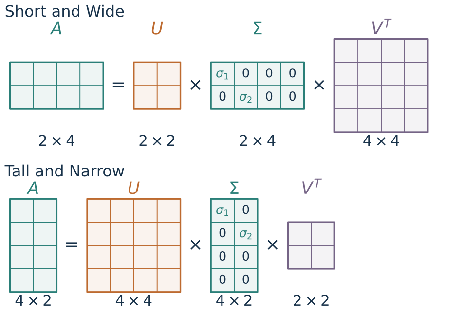
\(U\): square, sized by the rows of \(A\).

\(V^T\): square, sized by the columns of \(A\).

These are dimension diagrams, not numerical entries of a particular matrix. Each cell represents one entry. Both examples use the full SVD. The wide case has zero columns after Sigma’s two diagonal positions; the tall case has zero rows below them. Point out that U uses the output dimension m while V uses the input dimension d. Ask students to check the matrix products from right to left.

Singular values tell us how much each direction scales

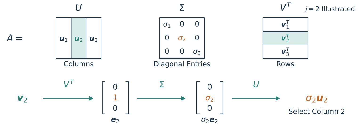
\[ V^T\boldsymbol{v}_j=\boldsymbol{e}_j \quad\Longrightarrow\quad A\boldsymbol{v}_j=U(\Sigma\boldsymbol{e}_j)=\sigma_j\boldsymbol{u}_j, \qquad j\le\min(m,d). \]

The diagram uses a square 3 by 3 example and j=2; the equation applies to full rectangular SVD with j <= min(m,d). Rows of V transpose compute v_i transpose v_j, which is 1 for i=j and 0 otherwise. Sigma produces sigma_j times the output-space basis vector; U selects its jth column. In rectangular cases the input and output basis vectors have lengths d and m respectively. Singular values above one stretch, below one shrink, and zero collapses a direction.

The largest singular value gives the maximum stretching

Order the singular values: \(\sigma_1\ge\sigma_2\ge\cdots\ge0\).

\[ \|A\boldsymbol{x}\|_2\le\sigma_1\|\boldsymbol{x}\|_2, \qquad \|A\|_2:=\max_{\|\boldsymbol{x}\|_2=1}\|A\boldsymbol{x}\|_2=\sigma_1. \]

• \(V^T\) and \(U\) preserve lengths.
• Each coordinate scaling in \(\Sigma\) is at most \(\sigma_1\).
• The input \(\boldsymbol{v}_1\) attains the largest scaling.

Introduce the operator or spectral norm as a maximum amplification, distinguishing it from the Euclidean norm of a vector. For a zero matrix the maximum is zero. The same bound applies to pairwise differences by linearity. Do not introduce condition numbers or optimization here.

Rank counts the independent directions that survive

\[ \operatorname{rank}(A)=\#\{j:\sigma_j>0\}\le\min(m,d) \]

For example:

\[ \Sigma=\begin{bmatrix}3&0&0\\0&1&0\\0&0&0\end{bmatrix} \qquad\Longrightarrow\qquad \operatorname{rank}(A)=2 \]

• Two independent input directions produce nonzero output directions.
• The third input direction disappears: \(A\boldsymbol{v}_3=\boldsymbol{0}\).
• Rotations and reflections change which directions these are, but not the rank.

Define rank as the dimension of the possible output space, then use the SVD to count that dimension. Rank belongs to an operator; do not confuse it with the number of distinct points in one finite dataset. Numerical near-zero thresholds come later; this slide concerns exact mathematical rank.