Linear Transformations and Reconstruction: Choosing a Decoder Basis

ECE 57000 — September 11, 2026

David I. Inouye

Wednesday made the SVD a way to read a linear transformation

• Orthogonal factors preserve lengths; singular values set directional scalings.
• The largest singular value bounds how much any input can stretch.
• Rank counts the nonzero singular values: how many independent directions survive.

Next question: When can we recover an input from its transformed output?

September 9 reached the rank slide after stakeholder-discovery guidance and the SVD interpretation. The recording ended after the rank example. Repeat that slide next, then develop null directions, recovery, and reconstruction. The recap is specific to this meeting and belongs only in the operational deck.

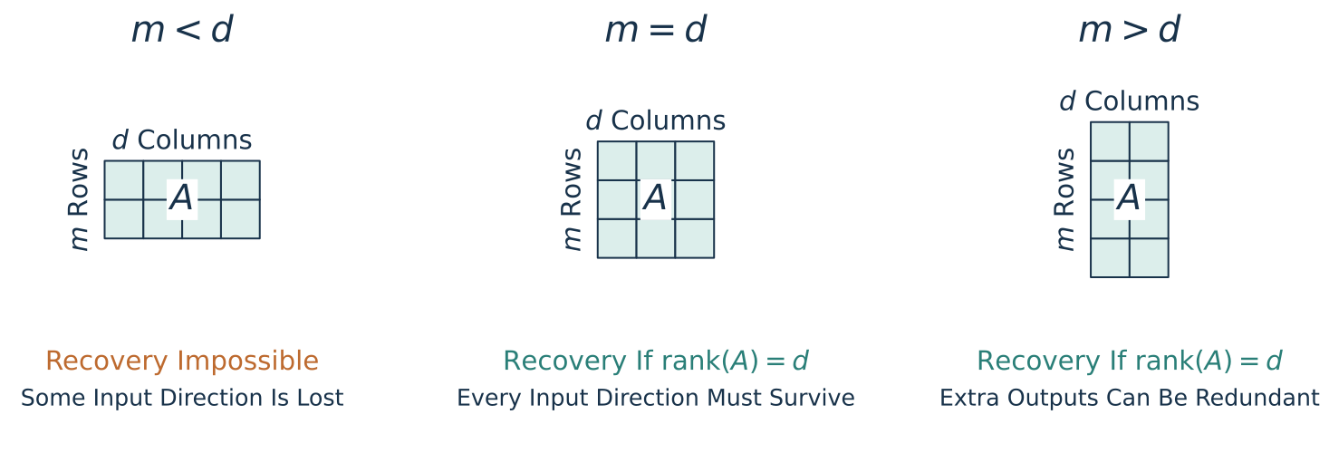
Rank counts the independent directions that survive

\[ \operatorname{rank}(A)=\#\{j:\sigma_j>0\}\le\min(m,d) \]

For example:

\[ \Sigma=\begin{bmatrix}3&0&0\\0&1&0\\0&0&0\end{bmatrix} \qquad\Longrightarrow\qquad \operatorname{rank}(A)=2 \]

• Two independent input directions produce nonzero output directions.
• The third input direction disappears: \(A\boldsymbol{v}_3=\boldsymbol{0}\).
• Rotations and reflections change which directions these are, but not the rank.

Define rank as the dimension of the possible output space, then use the SVD to count that dimension. Rank belongs to an operator; do not confuse it with the number of distinct points in one finite dataset. Numerical near-zero thresholds come later; this slide concerns exact mathematical rank.

A null direction makes different inputs indistinguishable

The null space contains all directions that map to zero:

\[ \operatorname{null}(A)=\{\boldsymbol{h}:A\boldsymbol{h}=\boldsymbol{0}\}. \]

For any nonzero \(\boldsymbol{h}\in\operatorname{null}(A)\):

\(\displaystyle A(\boldsymbol{x}+\boldsymbol{h})\)

\(=\)

\(\displaystyle A\boldsymbol{x}+A\boldsymbol{h}\)

(Distributivity)

\(\,\)

\(=\)

\(\displaystyle A\boldsymbol{x}\)

(Null direction)

The ambiguity is structural: any amount of movement along a null direction is invisible to the operator. It is not caused by a poor numerical algorithm.

A square operator is invertible when no direction collapses

In 1D, \(y=ax\) can be undone by \(x=y/a\) exactly when \(a\ne0\).

For square \(A=U\Sigma V^T\in\mathbb{R}^{d\times d}\):

\[ \text{all }\sigma_j>0 \quad\Longrightarrow\quad A^{-1}=V\Sigma^{-1}U^T, \qquad \Sigma^{-1}=\operatorname{diag}(1/\sigma_1,\ldots,1/\sigma_d). \]

\(\displaystyle A^{-1}A\)

\(=\)

\(\displaystyle (V\Sigma^{-1}U^T)(U\Sigma V^T)\)

(Substitute)

\(\,\)

\(=\)

\(\displaystyle V\Sigma^{-1}\Sigma V^T\)

(\(U^TU=I_d\))

\(\,\)

\(=\)

\(\displaystyle VV^T\)

(\(\Sigma^{-1}\Sigma=I_d\))

\(\,\)

\(=\)

\(\displaystyle I_d\)

(\(VV^T=I_d\))

The displayed computation verifies the proposed inverse. For a square matrix, a left inverse is also its inverse. An orthogonal factor is always invertible: Q inverse is Q transpose. Any failure of a square SVD to be invertible lies in a zero singular value. An invertible transformation may still distort distances; invertibility is not orthogonality.

Recovery depends on preserving every input direction

\(\boldsymbol{y}=A\boldsymbol{x}\) maps \(d\) input coordinates to \(m\) output coordinates.

Recovering every \(\boldsymbol{x}\in\mathbb{R}^d\) requires \(\operatorname{rank}(A)=d\).

The blocks show dimensions, not entries of specific matrices. Full column rank means no nonzero input is mapped to zero. More outputs permit this condition but do not guarantee it. A map with m<d can still distinguish a particular finite dataset or preserve a restricted subspace; the claim here concerns every input.

The pseudoinverse undoes every nonzero scaling

For any \(A=U\Sigma V^T\in\mathbb{R}^{m\times d}\), define:

\[ \underbrace{A^\dagger}_{d\times m} =\underbrace{V}_{d\times d}\underbrace{\Sigma^\dagger}_{d\times m}\underbrace{U^T}_{m\times m}. \]

\(\Sigma^\dagger\) has the transposed shape of \(\Sigma\), with zero off-diagonal entries:

\[ (\Sigma^\dagger)_{jj}= \begin{cases} 1/\sigma_j, & \sigma_j>0,\\ 0, & \sigma_j=0. \end{cases} \]

• Reverse the output reorientation, undo nonzero scalings, then reorient back.
• A zero scaling destroyed information; leaving it zero cannot restore it.
• The Moore–Penrose pseudoinverse exists even when \(A\) has no inverse.

For j up to min(m,d), reciprocate positive singular values and keep zero values zero; every other entry is zero. This defines the unique Moore–Penrose inverse regardless of nonuniqueness in SVD factors. It exists for every real matrix, including the zero matrix. If A is square and invertible, this is exactly the inverse formula just proved. Numerical thresholds for tiny singular values are a separate numerical-computation issue. No four-identity axiom list is needed for the conceptual role here. It is useful later for least squares, but not a prerequisite for deriving the PCA reconstruction objective.

The pseudoinverse recovers inputs exactly when no input direction is lost

For \(\boldsymbol{y}=A\boldsymbol{x}\), recovery of every input means:

\[ \widehat{\boldsymbol{x}}=A^\dagger\boldsymbol{y}=\boldsymbol{x} \ \text{for all }\boldsymbol{x}\in\mathbb{R}^d \quad\Longleftrightarrow\quad A^\dagger A=I_d. \]

Let \(r=\operatorname{rank}(A)\) and \(V_r=[\boldsymbol{v}_1\;\cdots\;\boldsymbol{v}_r]\) contain its surviving input directions.

\(\displaystyle A^\dagger A\)

\(=\)

\(\displaystyle V\Sigma^\dagger U^TU\Sigma V^T\)

(Substitute)

\(\,\)

\(=\)

\(\displaystyle V(\Sigma^\dagger\Sigma)V^T\)

(\(U^TU=I_m\))

\(\,\)

\(=\)

\(\displaystyle V_rV_r^T\)

(Keep nonzero directions)

\(\Sigma^\dagger\Sigma\) has \(r\) diagonal ones and \(d-r\) zeros. Thus \(A^\dagger A=I_d\) exactly when \(r=d\): full column rank, requiring \(m\ge d\).

Order singular values with positive values first. V_r V_r transpose keeps the component in the surviving input subspace and removes null-space components. If r=0, interpret this as the zero matrix. For a particular input outside this subspace, the lost component is unidentifiable from y. A reconstruction algorithm cannot recover every input from the same output when multiple inputs share it. More output coordinates only permit full column rank; they do not ensure it. The pseudoinverse exists regardless of whether this exact-recovery condition holds.

A restricted input subspace can be recovered exactly

Inputs: \(\boldsymbol{x}=t\boldsymbol{u}\in\mathbb{R}^2\), \(\|\boldsymbol{u}\|_2=1\). Encoder: \(A=\boldsymbol{v}^T\), with \(\alpha=\boldsymbol{v}^T\boldsymbol{u}\ne0\).

Decode with \(B=\boldsymbol{u}/\alpha\): knowing the line lets us undo its nonzero scaling.

\[ \widehat{\boldsymbol{x}}=By=\frac{\boldsymbol{u}}{\alpha}(\alpha t)=t\boldsymbol{u}=\boldsymbol{x}. \]

If \(\boldsymbol{v}=\boldsymbol{u}\), then \(\alpha=1\), \(y=t\), and \(B=A^\dagger=\boldsymbol{u}\). In general, \(B\ne A^\dagger\).

Ambient dimension is 2; intrinsic dimension is 1. Every nonperpendicular encoder direction v works: v^T u != 0 ensures distinct t give distinct outputs. If v is perpendicular to u, every point on the line maps to zero and recovery is impossible. The figure uses u=(0.8,0.6), v=(1,0), so alpha=0.8. B is the inverse of A restricted to the known line, not generally the Moore-Penrose pseudoinverse of A on the ambient space. For A=v^T, A^dagger=v/(vT v) selects the minimum-norm ambient solution, which generally lies along v rather than along the known input line u. BA acts as the identity on S even though BA != I_2. When v=u is unit length, B=A^dagger=u and y=t. More generally, recovery on a known subspace S is possible iff S intersects null(A) only at zero. A line through the origin is a linear subspace and a simple embedded manifold; shifted lines require an offset, and curved manifolds need not admit one global linear coordinate.

Read what an operator does from its singular values

A sensor-processing system uses \(A=U\operatorname{diag}(4,1,0)V^T\).

Can you recover every sensor input? What is the largest possible stretching factor? Could this operator preserve every pairwise distance? Explain which input direction is invisible to the system.

Rank \(2\); recovery is impossible in general; maximum scaling is \(4\). The direction \(\boldsymbol{v}_3\) disappears. All distances cannot be preserved.

Pairs, 3–4 minutes. Students must connect each claim to a singular value, not just name a property. Ask whether observing distinct outputs for a small test sample would overturn the recovery conclusion: it would not.

Data near a subspace can have small reconstruction error

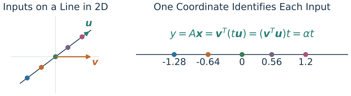
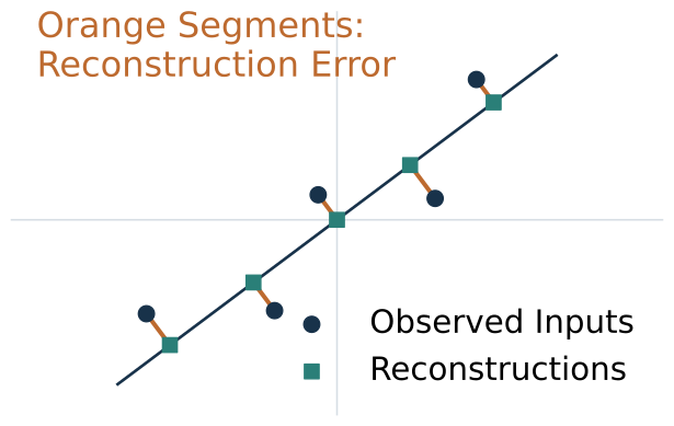
What if the inputs are close to a line, but do not lie exactly on it?

\[ y=\boldsymbol{u}^T\boldsymbol{x},\qquad \widehat{\boldsymbol{x}}=\boldsymbol{u}y,\qquad \text{error}=\|\boldsymbol{x}-\widehat{\boldsymbol{x}}\|_2^2. \]

Which direction minimizes total reconstruction error?

The exact line case has zero error. Near the line, each residual is perpendicular to the retained direction and is discarded by the encoder. Small residuals mean approximate recovery, not exact inversion. Here the line passes through the origin; the next topic centers observations before choosing a subspace. The figure is illustrative synthetic data. Do not claim that this displayed line is already the optimal PCA line; selecting that line is the coming problem.

Reconstruction and Principal Component Analysis

David I. Inouye

Dynamic Content · Last Updated: September 11, 2026

This topic formalizes dimensionality reduction through reconstruction, then derives PCA. It assumes the preceding topic’s SVD, rank, and recoverability results. Topic boundaries are conceptual; class meetings may stop within either topic.

A useful reduction should reconstruct the observed data well

Return to the cells described by many measured features.

• Fewer coordinates cannot preserve every possible input exactly.
• The observed data may nevertheless lie near a lower-dimensional subspace.
• We will judge a representation by how well it reconstructs those observations.

What reconstruction error are we willing to accept in exchange for fewer features?

Four steps lead to the PCA formulation

We will turn “reconstruct the data well” into a problem involving one matrix.

1. Define what a good reconstruction means — Next

Choose a representation size and measure reconstruction error.

2. Choose a convenient decoder basis.

An orthonormal basis can represent the same reconstruction subspace.

3. Find the best encoder for that decoder.

The closest point in the subspace determines the coordinates.

4. Formulate the subspace choice.

Combine these results into the PCA optimization problem.

Centering separates the mean from variation

For notation simplicity, we now call the raw data \(\widetilde X\) and the centered data \(X\).

\[ \boldsymbol{\mu}=\frac1n\sum_{i=1}^n\widetilde{\boldsymbol{x}}_i, \qquad X=\widetilde X-\boldsymbol{1}_n\boldsymbol{\mu}^T. \]

• Each row is \(\boldsymbol{x}_i^T=(\widetilde{\boldsymbol{x}}_i-\boldsymbol{\mu})^T\).
• Every feature column of \(X\) has mean zero.
• From here on, \(X\) and \(\boldsymbol{x}_i\) always denote centered data.

Add the mean back to reconstruct raw measurements: \(\widehat{\widetilde{\boldsymbol{x}}}_i=\boldsymbol{\mu}+\widehat{\boldsymbol{x}}_i\).

The preceding topic used X for general data. Announce this local notation change explicitly: tilde marks raw observations; unadorned symbols mean centered data. Both matrices have n rows and d columns. Define the all-ones vector 1_n and show its product with mu transpose repeats the mean row. Centering does not standardize different measurement units. In the cell example, preprocessing choices still determine what Euclidean error means.

A linear encoder and decoder make reconstruction explicit

For one centered observation, use the same operator convention as \(\boldsymbol{y}=A\boldsymbol{x}\):

\[ \boldsymbol{z}_i=\underbrace{E}_{k\times d}\boldsymbol{x}_i, \qquad \widehat{\boldsymbol{x}}_i=\underbrace{D}_{d\times k}\boldsymbol{z}_i. \]

Stacking observations as rows gives:

\[ \underbrace{Z}_{n\times k} =\underbrace{X}_{n\times d}\underbrace{E^T}_{d\times k}, \qquad \underbrace{\widehat X}_{n\times d} =\underbrace{Z}_{n\times k}\underbrace{D^T}_{k\times d}. \]

The batch reconstruction is \(\widehat X=XE^TD^T\), with rank at most \(k\).

D here is a general decoder, not the diagonal matrix from the earlier operator examples. The rank-at-most-k requirement comes from passing through k features. Do not assume D equals E transpose at this stage.

Reconstruction error formalizes one meaning of preservation

Choose a linear encoder and decoder to minimize squared reconstruction error:

\[ \min_{E,D}\|X-XE^TD^T\|_F^2. \]

The Frobenius norm measures the error across every entry:

\[ \|M\|_F^2=\sum_{i,j}M_{ij}^2, \qquad \|X-\widehat X\|_F^2 =\sum_{i=1}^n\|\boldsymbol{x}_i-\widehat{\boldsymbol{x}}_i\|_2^2. \]

Bridge the new matrix norm by summing the familiar vector squared error across observations. The objective treats measured coordinates according to their scale; it does not automatically encode biological meaning or downstream usefulness.

Four steps lead to the PCA formulation

We have an error measure. Now consider which reconstructions the decoder can produce.

1. Define what a good reconstruction means — Established

Choose a representation size and measure reconstruction error.

2. Choose a convenient decoder basis — Next

An orthonormal basis can represent the same reconstruction subspace.

3. Find the best encoder for that decoder.

The closest point in the subspace determines the coordinates.

4. Formulate the subspace choice.

Combine these results into the PCA optimization problem.

Matrix–vector multiplication combines the matrix’s columns

For a \(3\times2\) decoder, the familiar row dot products can be regrouped by column:

\[ \begin{bmatrix}d_{11}&d_{12}\\d_{21}&d_{22}\\d_{31}&d_{32}\end{bmatrix} \begin{bmatrix}z_1\\z_2\end{bmatrix} = \underbrace{\begin{bmatrix}d_{11}z_1+d_{12}z_2\\d_{21}z_1+d_{22}z_2\\d_{31}z_1+d_{32}z_2\end{bmatrix}}_{\text{one dot product per row}} = z_1\underbrace{\begin{bmatrix}d_{11}\\d_{21}\\d_{31}\end{bmatrix}}_{\boldsymbol{d}_1} +z_2\underbrace{\begin{bmatrix}d_{12}\\d_{22}\\d_{32}\end{bmatrix}}_{\boldsymbol{d}_2}. \]

For any number of columns: \(\widehat{\boldsymbol{x}}=D\boldsymbol{z}=\sum_{j=1}^k z_j\boldsymbol{d}_j\).

• Let \(\boldsymbol{z}\) be arbitrary for now. Every reconstruction lies in \(\mathcal{S}=\operatorname{span}\{\boldsymbol{d}_1,\ldots,\boldsymbol{d}_k\}\).
• First choose how \(D\) describes that subspace; then choose the best coordinates.

Point to each entry in the middle vector, then collect all z1 terms into the first column and all z2 terms into the second. These are two interpretations of the same multiplication. Column vectors d_j live in the original d-dimensional space. No encoder has been chosen: z is any vector in R^k. The decoder limits where a reconstruction can lie regardless of how z is produced. All inputs in this topic are centered; observations are stacked as rows only in batch formulas.

Scaling a decoder direction only changes its coordinates

A line can use a unit vector \(\boldsymbol{u}\) or the scaled vector \(3\boldsymbol{u}\).

\[ \underbrace{\boldsymbol{u}}_{\text{unit basis}}\underbrace{t}_{\text{coordinate}} = \underbrace{(3\boldsymbol{u})}_{\text{scaled basis}}\underbrace{(t/3)}_{\text{adjusted coordinate}}. \]

Both describe the same point on the same line.

• A nonzero column can be normalized if we rescale its coordinate to compensate.
• Unit columns remove an arbitrary scale choice; no reconstruction is lost.
• Next: can we choose perpendicular columns while keeping the same subspace?

This is a parameterization choice, not a claim that unit vectors reconstruct better than scaled ones. For column d_j=c_j w_j with c_j=norm(d_j)>0, d_j z_j=w_j(c_j z_j). Zero columns contribute nothing. Normalization alone does not make different columns perpendicular; address that separately next.

Perpendicular unit directions can describe the same subspace

Both unit-vector pairs span the plane: either represents every \(\boldsymbol{x}=[x_1,x_2]^T\).

For \(\boldsymbol{b}_1=[1,0]^T\), \(\boldsymbol{b}_2=[1,1]^T/\sqrt2\):

\[ \boldsymbol{x}=(x_1-x_2)\boldsymbol{b}_1+\sqrt2\,x_2\boldsymbol{b}_2. \]

For \(\boldsymbol{w}_1=[1,0]^T\), \(\boldsymbol{w}_2=[0,1]^T\):

\[ \boldsymbol{x}=(\boldsymbol{w}_1^T\boldsymbol{x})\boldsymbol{w}_1 +(\boldsymbol{w}_2^T\boldsymbol{x})\boldsymbol{w}_2. \]

Same plane; simpler coordinates: an orthonormal basis gives each coefficient by a dot product.

The retained plane is drawn face-on. Both panels show the same point [2,1]^T. Left: b1=[1,0]^T, b2=[1,1]^T/sqrt(2), so x=b1+sqrt(2)b2. Right: x=2w1+w2. For any x=[x1,x2]^T, expanding (x1-x2)b1+sqrt(2)x2 b2 gives [x1,x2]^T. Thus both independent unit pairs span the entire plane, not only this example. For a skew unit basis, b1^T x=z1+(b1^T b2)z2; b2^T x=(b2^T b1)z1+z2. Individual dot products mix coefficients. Dividing by each basis vector’s squared norm does not undo that mixing. For an orthogonal non-unit basis, z_j=(b_j^T x)/(b_j^T b_j) does work; orthonormality also removes the denominator. Every subspace admits an orthonormal basis. It is not unique; changing the basis changes coordinates, not reconstruction possibilities. The next slide formalizes how to absorb the coordinate change into the encoder.

QR lets us choose an orthonormal decoder without changing reconstruction

Start with any encoder \(E_0\in\mathbb{R}^{k\times d}\) and decoder \(D_0\in\mathbb{R}^{d\times k}\), where \(k\le d\). Suppose \(D_0\) does not have orthonormal columns.

The thin QR decomposition writes \(D_0=WR\): \(W^TW=I_k\) and \(R\) is upper triangular. Here \(W\in\mathbb{R}^{d\times k}\) and \(R\in\mathbb{R}^{k\times k}\).

Can we choose \(D=W\) and a new \(E\) to keep every reconstruction the same?

\(\displaystyle D_0E_0\boldsymbol{x}\)

\(=\)

\(\displaystyle (WR)E_0\boldsymbol{x}\)

(QR of the original decoder)

\(\,\)

\(=\)

\(\displaystyle W(RE_0)\boldsymbol{x}\)

(Regroup the factors)

\(\,\)

\(=\)

\(\displaystyle DE\boldsymbol{x}\)

(Choose \(D=W\), \(E=RE_0\))

Same reconstruction for every input: an orthonormal decoder is without loss of generality. Next, fix \(D=W\) and find its best encoder.

Introduce both original operators before factoring the decoder. QR is another standard matrix decomposition, introduced here because it solves a specific problem. The factor usually named Q is called W to match our subspace notation. In thin QR for d by k with k<=d, W has k orthonormal columns and R is k by k upper triangular (entries below the diagonal are zero). If D0 has full column rank, W is a basis of exactly its column span and R is invertible. Thin QR also exists for deficient rank: W spans a k-dimensional space containing the decoder span, and R is singular. We never invert R, so the reconstruction identity holds in either case. For a general rectangular matrix, full QR uses a square orthogonal Q and an upper-trapezoidal R; avoid saying every rectangular R is square triangular. We do not need to teach the QR algorithm here. Triangularity is a property of this standard factorization, not needed for the regrouping. The new encoder RE0 remains arbitrary; its optimal choice W^T is derived next. With row-stacked inputs the identity is X E0^T D0^T = X E^T D^T.