PCA Interpretation and NumPy Computation

ECE 57000 — September 18, 2026

David I. Inouye

Wednesday proved which PCA subspace is optimal

• For centered data, minimizing reconstruction error is equivalent to maximizing \(\|XW\|_F^2\).
• Every orthonormal \(W\) retains at most \(\sum_{j=1}^k\sigma_j^2\); choosing \(W=V_k\) attains that bound.
• The discarded squared singular values give reconstruction error: \(\|X-X_k\|_F^2=\sum_{j>k}\sigma_j^2\).
• Each PCA coordinate has sample variance \(\sigma_j^2/(n-1)\); choosing \(k\) still depends on the intended use.

Next: revisit the variance interpretation, finish PCA’s geometric interpretation, then implement it in NumPy.

Squared singular values give the variance of each PCA coordinate

The \(j\)th coordinate across observations is \(Z_{:j}=X\boldsymbol{v}_j=\sigma_j\boldsymbol{u}_j\). Since \(X\) is centered, this coordinate also has mean zero.

\(\displaystyle \operatorname{Var}_{\mathrm{sample}}(Z_{:j})\)

\(=\)

\(\displaystyle \frac{1}{n-1}\sum_{i=1}^n Z_{ij}^2\)

(Variance of a centered coordinate; \(n>1\))

\(\,\)

\(=\)

\(\displaystyle \frac{\sigma_j^2}{n-1}\|\boldsymbol{u}_j\|_2^2\)

(Substitute \(Z_{:j}=\sigma_j\boldsymbol{u}_j\))

\(\,\)

\(=\)

\(\displaystyle \frac{\sigma_j^2}{n-1}\)

(\(\boldsymbol{u}_j\) is a unit vector)

The leading PCA coordinates therefore have the largest variances. This interprets the solution we already proved.

Define Z_{:j} as column j of Z, containing one scalar coordinate per observation. It is centered because sum_i x_i=0 implies sum_i v_j^T x_i=0. Sample variance divides the sum of squared centered entries by n-1. Work with j<=k<=r as in the truncated factor slide. We are naming the statistical meaning of squared length, not proving the reconstruction/retained-energy equivalence again.

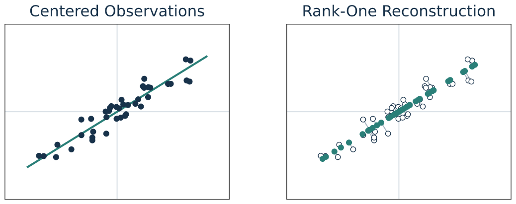
One retained direction can reconstruct a narrow data cloud

Original-scale reconstruction: \(\widehat{\widetilde{\boldsymbol{x}}}_i=\boldsymbol{\mu}+W\boldsymbol{z}_i\).

Synthetic example, not cell measurements. The second panel shows reconstruction back in two dimensions, not the one-dimensional feature coordinate itself. The short perpendicular segments are exactly the errors the PCA objective measures.

A curved structure can be low-dimensional without being linear

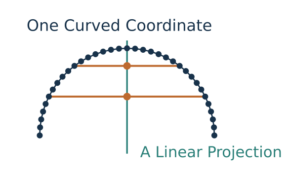
Would one linear feature reconstruct every point exactly? Could a nonlinear coordinate do so? What does “one-dimensional” mean in each claim?

Pairs, 3 minutes. A curved arc can be parameterized by one angle, but no straight line contains it, so one-dimensional linear reconstruction cannot be exact. This particular vertical projection also creates collisions; do not claim every linear projection of a semicircle has collisions. A horizontal coordinate on this upper semicircle is injective, but its exact decoder would be nonlinear.

PCA solves the stated problem; usefulness still needs evidence

• Chosen objective: squared error in the selected measurements and units.
• Mathematical solution: leading right singular vectors of centered data.
• Remaining questions: which features and preprocessing, how many components, and whether the retained variation matters for the intended use.

Next: translate this mathematical contract into arrays and reliable numerical computation—then ask what the observed data justify claiming about new cases.

Return to the cell-expression anchor: a faithful reconstruction is evidence for this proxy, not automatically for cell type, biological mechanism, or future prediction. Stop the math section here; the next topic introduces NumPy, vectorization, numerical stability, and empirical interpretation.

NumPy and Numerical Computation for PCA

David I. Inouye

Dynamic Content · Last Updated: September 17, 2026

Draft for instructor review. Assumes the completed reconstruction/PCA topic: centering, orthonormal projection, SVD, and the discarded-energy formula. The outline lives in redesign/arc-02-formalization-representation.md. This is a conceptual topic, not a commitment to one class meeting.

The PCA equations give us a computation to implement

Let \(\widetilde X\in\mathbb R^{n\times d}\) contain the original observations as rows.

Operation	Mathematics	Shape
Center	\(X=\widetilde X-\boldsymbol{1}\boldsymbol{\mu}^T\)	\(n\times d\)
Choose directions	\(X=U\Sigma V^T\), \(W=V_k\)	\(d\times k\)
Encode	\(Z=XW\)	\(n\times k\)
Reconstruct	\(\widehat{\widetilde X}=ZW^T+\boldsymbol{1}\boldsymbol{\mu}^T\)	\(n\times d\)

Route: represent the objects, implement the operations, check the numerical result.

Use real-valued finite measurements throughout, n>1 and 1<=k<=min(n,d). The vector of ones has n entries. In code, A represents original data and X represents centered data, preserving the preceding topic’s meaning of X. The mean is estimated column by column. NumPy details serve these equations.

Lists and arrays give different meanings to *

import numpy as np

values = [2, 5, 8]
x = np.array(values, dtype=np.float64)

print("type(values):", type(values))
print("type(x):", type(x))
print(f"values * 2: {values * 2!r}")
print(f"x * 2: {x * 2!r}")
print("x.shape:", x.shape)
print("x.dtype:", x.dtype)

type(values): <class 'list'>
type(x): <class 'numpy.ndarray'>
values * 2: [2, 5, 8, 2, 5, 8]
x * 2: array([ 4., 10., 16.])
x.shape: (3,)
x.dtype: float64

• A list is a Python sequence. Multiplication by an integer repeats it.
• An array stores values with a common data type. Here multiplication scales each entry.
• shape describes the axes. dtype describes how entries are stored.

This is the minimum container bridge, not a general Python tutorial. Use float64 explicitly in these examples so precision comparisons are deliberate. [Sources] source:numpy-array-basics-2026 — array creation, shape, and dtype.

A one-dimensional array has no row or column axis to swap

Shapes: (d,) = one observation; (n, d) = observations × features; (b, n, d) adds a batch axis.

x = np.array([2., 5., 8.])
print("x.shape:", x.shape)
print("x.T.shape:", x.T.shape)
print("x[:, None].shape:", x[:, None].shape)
print("x[None, :].shape:", x[None, :].shape)

x.shape: (3,)
x.T.shape: (3,)
x[:, None].shape: (3, 1)
x[None, :].shape: (1, 3)

• None (equivalently np.newaxis) inserts a length-one axis at that position.
• x[:, None] makes a column; x[None, :] makes a row.
• For 2D arrays, .T swaps the row and column axes.

Indexing: A[i, :] selects observation \(i\); A[:, j] selects feature \(j\).

None inserts an axis of length one. Distinguish a mathematical vector’s role from its storage convention. Keep all PCA batches explicitly two-dimensional. [Sources] source:numpy-array-basics-2026 — adding axes and transposing arrays.

* multiplies entries; @ implements matrix multiplication

P = np.array([[1., 2.],
              [3., 4.]])
Q = np.array([[2., 0.],
              [1., 2.]])
print("P * Q (entrywise):\n", P * Q)
print("P @ Q (matrix product):\n", P @ Q)

P * Q (entrywise):
 [[2. 0.]
 [3. 8.]]
P @ Q (matrix product):
 [[ 4.  4.]
 [10.  8.]]

For PCA, Z = X @ W maps (n, d) @ (d, k) to (n, k).

The upper-left entries are \(1\cdot2=2\) and \(1\cdot2+2\cdot1=4\). Both results have shape (2, 2). Shape alone cannot tell us which operation we intended.

Centering averages across observations for each feature

For each feature, \(\mu_j=\frac1n\sum_{i=1}^n\widetilde X_{ij}\).

A = np.array([[2., 10.],
              [4., 14.], [6., 18.]])
mu = A.mean(axis=0)
X = A - mu
print("mu (feature means):", mu)
print("X (centered data):\n", X)

mu (feature means): [ 4. 14.]
X (centered data):
 [[-2. -4.]
 [ 0.  0.]
 [ 2.  4.]]

Axis rule: count positions in the shape tuple from zero. Aggregate over the chosen dimension and remove it by default. The resulting shapes are:

T = np.zeros((2, 3, 4))
print("T.shape:", T.shape)
print("axis=0:", T.mean(axis=0).shape)
print("axis=1:", T.mean(axis=1).shape)
print("axis=2:", T.mean(axis=2).shape)

T.shape: (2, 3, 4)
axis=0: (3, 4)
axis=1: (2, 4)
axis=2: (2, 3)

Why does X = A - mu work? Ordinary matrix subtraction requires equal shapes. A matrix minus a vector is undefined. NumPy supplies broadcasting.

Trace the first column numerically before considering the whole matrix. Do not imply these synthetic values are actual cell measurements. For A, axis=0 aggregates observations and leaves features; axis=1 would aggregate features within each observation. For T, point to positions 0, 1, and 2 of (2,3,4): removing them gives (3,4), (2,4), and (2,3). Zeros keep attention on shapes rather than values. These output shapes use the default keepdims=False; the broadcasting section introduces keepdims=True. [Sources] source:numpy-array-basics-2026 — reductions over axes.

Broadcasting compares dimensions from right to left

At each position, either of two rules must hold:

1. The two dimension sizes are equal: keep that size.
2. One size is 1: reuse its value along the other dimension’s size.

Missing dimensions count as 1s (marked * below). If neither rule holds at any position, broadcasting fails.

Vector (4,)

(3, 4)
(*, 4)
------
(3, 4)

Matrix (3, 1)

(2, 3, 4)
(*, 3, 1)
---------
(2, 3, 4)

Both inputs expand

(3, 1)
(1, 4)
------
(3, 4)

Scalar ()

(2, 3, 4)
(*, *, *)
---------
(2, 3, 4)

Vector (3,): incompatible

(3, 4)
(*, 3)
------
 Error

Rightmost sizes 4 and 3 are neither equal nor 1.

Point to the rightmost pair first in every row. Missing dimensions mean missing leading positions after right alignment, not arbitrary gaps between axes. For (2,3,4) and (3,1): compare 4 with 1, then 3 with 3, then 2 with a missing 1. Dimension sizes in these teaching examples are positive. The star is a diagram placeholder, not literal NumPy shape syntax. Raw input shapes are shown above each stack; placeholders make absent leading axes visible. [Sources] source:numpy-broadcasting-2026 — general broadcasting rules.

Mathematics makes the repeated mean an explicit matrix

\[ \underbrace{X}_{n\times d} =\underbrace{\widetilde X}_{n\times d} -\underbrace{\boldsymbol{1}_n\boldsymbol{\mu}^T}_{(n\times1)(1\times d)=n\times d}. \]

In NumPy, A - mu produces the same entries: \(X_{ij}=\widetilde X_{ij}-\mu_j\).

ones = np.ones((A.shape[0], 1))
mu_matrix = ones @ mu[None, :]
print("mu_matrix:\n", mu_matrix)
print("A - mu:\n", A - mu)
print("Same result:",
      np.allclose(A - mu_matrix, A - mu))

mu_matrix:
 [[ 4. 14.]
 [ 4. 14.]
 [ 4. 14.]]
A - mu:
 [[-2. -4.]
 [ 0.  0.]
 [ 2.  4.]]
Same result: True

A: (3, 2); mu: (2,). Broadcasting avoids copying the repeated means, saving allocation and memory traffic. The output still needs storage.

The vector of ones makes the subtraction well-defined in ordinary matrix algebra. Its product with the row vector of feature means repeats that row n times. We construct it here only to connect the equation with the broadcast computation. np.allclose checks the agreement on this example; the entrywise identity explains why they agree generally. The output X still needs n-by-d storage. [Sources] source:numpy-broadcasting-2026 — conceptual expansion without copying operands.

keepdims=True preserves reduced axes with length one

For T.shape == (2, 3, 4), reducing axis=1 gives (2, 4) by default. With keepdims=True, it gives (2, 1, 4): the reduced position stays explicit.

reduced = T.mean(axis=1)
kept = T.mean(axis=1, keepdims=True)
restored = reduced[:, None, :]
print("T.shape:", T.shape)
print("reduced.shape:", reduced.shape)
print("kept.shape:", kept.shape)
print("restored.shape:", restored.shape)
print("(T - kept).shape:", (T - kept).shape)

T.shape: (2, 3, 4)
reduced.shape: (2, 4)
kept.shape: (2, 1, 4)
restored.shape: (2, 1, 4)
(T - kept).shape: (2, 3, 4)

• keepdims preserves a reduced axis; None inserts a new axis where specified.
• (2, 1, 4) broadcasts back against (2, 3, 4).
• (2, 4) would align as (1, 2, 4) and fail at the middle position.

The mean values are the same in reduced, kept, and restored; their shapes differ. Use the zero-valued tensor from the earlier axis example so only the shapes are at issue. Indexing with None or np.newaxis inserts a view axis rather than repeating values. The missing middle singleton cannot be inferred by the right-to-left rule; only missing leading positions receive implicit ones. [Sources] source:numpy-array-basics-2026 — adding axes and keeping reduced dimensions. source:numpy-broadcasting-2026 — alignment from the right.

Division broadcasts one standard deviation per feature

For positive feature standard deviations \(s_j\), \(H_{ij}=(\widetilde X_{ij}-\mu_j)/s_j\). In matrix notation, \(H=X\operatorname{diag}(1/s_1,\ldots,1/s_d)\).

std = A.std(axis=0)
H = (A - mu) / std
H_mul = (A - mu) * (1 / std)
print("std:", std.round(3))
print("H.round(3):\n", H.round(3))
print("H.std(axis=0):", H.std(axis=0))
print("Division equals multiplication:",
      np.allclose(H, H_mul))

std: [1.633 3.266]
H.round(3):
 [[-1.225 -1.225]
 [ 0.     0.   ]
 [ 1.225  1.225]]
H.std(axis=0): [1. 1.]
Division equals multiplication: True

(3, 2) / (2,) reuses each feature’s scale across observations. The same shape rules apply to elementwise +, -, *, and /. Scaling changes the relative weight of features in PCA’s reconstruction error.

This example uses NumPy’s default ddof=0, dividing variance by n. Both columns have positive standard deviation. A constant feature needs separate treatment before division. The arithmetic illustrates broadcasting, not a recommendation that all gene-expression features should be standardized. Scaling changes the PCA objective by weighting squared errors inversely by feature scale squared. Matrix @ has its own contracted-dimension rules; do not apply elementwise rules to those axes. [Sources] source:numpy-broadcasting-2026 — elementwise arithmetic with broadcast operands.

Code can run successfully while centering the wrong objects

A = np.array([[2., 10.],
              [4., 14.], [6., 18.]])
B = A - A.mean(axis=1, keepdims=True)
print("B:\n", B)
print("B.mean(axis=1):", B.mean(axis=1))
print("B.mean(axis=0):", B.mean(axis=0))

B:
 [[-4.  4.]
 [-5.  5.]
 [-6.  6.]]
B.mean(axis=1): [0. 0. 0.]
B.mean(axis=0): [-5.  5.]

What does this code subtract? Which averages become zero? Would this prepare the data for the PCA problem we defined? Repair the expression and explain why.

Pairs, 3 minutes plus a short debrief. Diagnose meaning rather than syntax. The code subtracts each observation’s average across its two features. Every row mean is zero, while the feature means need not be zero. Repair with axis=0, with or without keepdims. Distinct n and d prevent an accidental square-matrix match from distracting from the conceptual error.

NumPy returns the right singular vectors as rows of Vt

U, s, Vt = np.linalg.svd(
    X, full_matrices=False)
W = Vt[:k, :].T

full_matrices=False omits extra directions multiplied by zero rows or columns of rectangular \(\Sigma\). This reduced SVD keeps \(m=\min(n,d)\) singular values; selecting the first \(k\) is a separate truncation.

Returned array	Shape	Mathematical role
U	(n, m)	Left singular vectors
s	(m,)	Singular values, largest first
Vt	(m, d)	Rows are right singular vectors transposed
W	(d, k)	First \(k\) right singular vectors as columns

The argument False requests reduced shapes, not a rank-k approximate solver. The routine still computes all min(n,d) singular values. Rank may be smaller than m. We restrict k to 1..m. For complex input the output is the conjugate transpose, but this lecture uses real data. The variable name Vt is our choice. [Sources] source:numpy-svd-2026 — return values and full_matrices.

Encoding and reconstruction follow the same equations as before

Xraw stores \(\widetilde X\), the original observations.

Xraw = np.array([[2., 10.], [4., 15.],
                 [6., 17.], [8., 22.]])
mu = Xraw.mean(axis=0)
X = Xraw - mu
U, s, Vt = np.linalg.svd(
    X, full_matrices=False)
k = 1
W = Vt[:k, :].T
Z = X @ W
Xraw_hat = Z @ W.T + mu
print("Z.round(3):\n", Z.round(3))

Z.round(3):
 [[-6.708]
 [-1.347]
 [ 1.347]
 [ 6.708]]

For \(X\in\mathbb R^{n\times d}\) and \(W\in\mathbb R^{d\times k}\), \(\widehat X=(XW)W^T=X(WW^T)\).

Centered reconstruction	Arithmetic cost	Intermediate
Xhat = (X @ W) @ W.T	\(O(ndk)\)	\(n\times k\)
Xhat = X @ (W @ W.T)	\(O(d^2k+nd^2)\)	\(d\times d\)

This is the complete small dense PCA computation, with finite real input and valid k assumed. Ask students to identify the encoder and decoder. Vectorization: X @ W computes all observations together. With standard dense multiplication, the first grouping costs ndk + nkd = 2ndk operations up to constant factors. The second costs dkd + ndd. For k much smaller than d, using the coordinates avoids the large d-by-d projection matrix. Costs exclude the preceding SVD and restoring the mean; Xhat here is centered. Subtracting the original-scale arrays measures the same residual as X-Z@W.T. [Sources] source:numpy-svd-2026 — reduced SVD reconstruction.

The computed arrays show PCA’s shapes and reconstruction

print("X.shape:", X.shape)
print("U.shape:", U.shape)
print("s.shape:", s.shape)
print("Vt.shape:", Vt.shape)
print("W.shape:", W.shape)
print("Z.shape:", Z.shape)
print("Xraw_hat.shape:", Xraw_hat.shape)
print("s.round(4):", s.round(4))
print("Xraw_hat.round(3):\n",
      Xraw_hat.round(3))
error = np.sum((Xraw - Xraw_hat)**2)
print(f"error (squared): {error:.6f}")

X.shape: (4, 2)
U.shape: (4, 2)
s.shape: (2,)
Vt.shape: (2, 2)
W.shape: (2, 1)
Z.shape: (4, 1)
Xraw_hat.shape: (4, 2)
s.round(4): [9.6755 0.6201]
Xraw_hat.round(3):
 [[ 1.923 10.04 ]
 [ 4.382 14.803]
 [ 5.618 17.197]
 [ 8.077 21.96 ]]
error (squared): 0.384552

We retained one direction, but full_matrices=False still computed both singular values.

Continue the preceding four-observation, two-feature example. Reduced factor shapes are distinct from a solver that computes only k components. [Sources] source:numpy-svd-2026 — reduced SVD shapes.

New observations use the fitted mean and directions

# Apply the representation fitted on Xraw
Xraw_new = np.array([[5., 16.], [7., 20.]])
Z_new = (Xraw_new - mu) @ W
Xraw_new_hat = Z_new @ W.T + mu
print("Z_new.round(3):\n", Z_new.round(3))
print("Xraw_new_hat.round(3):\n",
      Xraw_new_hat.round(3))

Z_new.round(3):
 [[0.   ]
 [4.472]]
Xraw_new_hat.round(3):
 [[ 5.    16.   ]
 [ 7.051 19.974]]

• Fitting estimates mu and W from a chosen dataset.
• Applying uses those fixed values for other observations with the same feature definitions.
• Re-estimating the mean or directions creates a different fitted representation.

PCA relies on centering and then measuring variance. What would happen if we computed variance directly, without centering first?

Students have not yet studied train/validation/test methodology. Establish the fit/apply distinction now, then let Arc 3 justify independent evaluation. If optional feature scaling is used, save and reuse the fitted scales as well.