Interpreting PCA and Formalizing Prediction

ECE 57000 — September 21, 2026

David I. Inouye

Friday connected PCA’s equations to working NumPy code

• PCA’s leading directions minimize reconstruction error and maximize retained variance; usefulness depends on the data and purpose.
• Array shapes, reduction axes, and broadcasting determine which computation the code performs.
• Center the observations, compute the reduced SVD, then encode with X @ W and reconstruct with Z @ W.T + mu.
• Reuse the fitted mean and directions for new observations; changing matrix-product grouping can greatly change memory and computation costs.

Today: can mathematically equivalent formulas give different numerical answers? Then return to real gene-expression data and ask what PCA reveals.

New observations use the fitted mean and directions

# Apply the representation fitted on Xraw
Xraw_new = np.array([[5., 16.], [7., 20.]])
Z_new = (Xraw_new - mu) @ W
Xraw_new_hat = Z_new @ W.T + mu
print("Z_new.round(3):\n", Z_new.round(3))
print("Xraw_new_hat.round(3):\n",
      Xraw_new_hat.round(3))

Z_new.round(3):
 [[0.   ]
 [4.472]]
Xraw_new_hat.round(3):
 [[ 5.    16.   ]
 [ 7.051 19.974]]

• Fitting estimates mu and W from a chosen dataset.
• Applying uses those fixed values for other observations with the same feature definitions.
• Re-estimating the mean or directions creates a different fitted representation.

PCA relies on centering and then measuring variance. What would happen if we computed variance directly, without centering first?

Students have not yet studied train/validation/test methodology. Establish the fit/apply distinction now, then let Arc 3 justify independent evaluation. If optional feature scaling is used, save and reuse the fitted scales as well.

Computing spread for PCA starts with an exact identity

For one feature’s values \(x_1,\ldots,x_n\), let \(\bar x=\frac1n\sum_{i=1}^{n}x_i\). The mean \(\bar x\) is constant with respect to \(i\).

\(\displaystyle \frac1n\sum_{i=1}^{n}(x_i-\bar x)^2\)

\(=\)

\(\displaystyle \frac1n\sum_{i=1}^{n}\bigl(x_i^2-2x_i\bar x+\bar x^2\bigr)\)

(Expand the square inside the sum)

\(\,\)

\(=\)

\(\displaystyle \frac1n\sum_{i=1}^{n}x_i^2-\frac{2\bar x}{n}\sum_{i=1}^{n}x_i+\frac1n\sum_{i=1}^{n}\bar x^2\)

(Distribute the sum; pull out constants)

\(\,\)

\(=\)

\(\displaystyle \frac1n\sum_{i=1}^{n}x_i^2-\frac{2\bar x}{n}(n\bar x)+\frac1n(n\bar x^2)\)

(\(\sum_{i=1}^{n}x_i=n\bar x\); \(n\) copies of \(\bar x^2\))

\(\,\)

\(=\)

\(\displaystyle \frac1n\sum_{i=1}^{n}x_i^2-2\bar x^2+\bar x^2\)

(Cancel the factors of \(n\))

\(\,\)

\(=\)

\(\displaystyle \frac1n\sum_{i=1}^{n}x_i^2-\bar x^2\)

(Combine terms)

Motivate from PCA: our mathematical variance interpretation and centering step now have to be evaluated on a finite-precision computer. Is algebraic correctness enough? Reduce to one feature and five numbers; this is the only worked failure. This is the average squared deviation of a finite list, using divisor n, not an expectation over a probability distribution or the n-1 sample estimator. Every sum runs from 1 through n. Explicitly point out that the constant term occurs n times. Reveal one algebraic operation at a time before asking whether its numerical implementations will agree.

Will mathematically equivalent computations give the same answer?

Take the five numbers \(10^9+1,\ldots,10^9+5\). Their mean is \(10^9+3\). What variances will the two computations report? Predict before revealing.

v = 1e9 + np.arange(1., 6.)
centered = v - v.mean()
center_first = np.mean(centered**2)
subtract_totals = np.mean(v**2) - v.mean()**2
print("Centered:", center_first)
print("Raw squares:", subtract_totals)

Centered: 2.0
Raw squares: 0.0

Choice	Centered	Raw squares
A	\(2\)	\(2\) (up to a tiny rounding error)
B	\(2\)	\(0\)
C	\(2\)	Overflow: the squared values are too large

Individual prediction, then a short pair discussion (about two minutes). Vote A, B, or C, then reveal the labeled outputs. B is correct. A expresses the expectation that any numerical difference must be tiny; C confuses loss of precision with exceeding the representable range. These squared values are within float64’s range: this example loses a small difference, not range. Both formulas are exactly equal in real arithmetic. On this float64 example the first gives 2.0 and the second 0.0. The original numbers are exactly representable; the failure occurs in computing the large squared quantities. Do not introduce another example or a different PCA solver.

Numerical errors can erase the entire answer

print("Centered values:", centered)
print("Mean of squares:", np.mean(v**2))
print("Square of mean:", v.mean()**2)
print("Centered:", center_first)
print("Raw squares:", subtract_totals)

Centered values: [-2. -1.  0.  1.  2.]
Mean of squares: 1.000000006e+18
Square of mean: 1.000000006e+18
Centered: 2.0
Raw squares: 0.0

• Centering first gives \((-2,-1,0,1,2)\): the mean square is \((4+1+0+1+4)/5=2\).
• The other formula subtracts rounded values near \(10^{18}\). The small difference is lost: catastrophic cancellation.
• This is 100% relative error: zero instead of two, not just a changed last decimal.

Numerical stability: choose computations that control the effect of rounding errors. A correct mathematical formula alone does not ensure a reliable computation.

Later: log probabilities help avoid tiny probabilities rounding to zero; softmax needs careful implementation to avoid overflow.

The two large computed terms round to the same float64 number in this example. Subtraction exposes the lost information; it cannot recover it. Centering first avoids the large intermediate squares here. It does not recover information already rounded away in input data. Keep the discussion at the principle level: mathematical equivalence does not guarantee numerical equivalence. This is the first explicit math-versus-computation lesson: numbers have finite precision, intermediate results are rounded, and the final error can be large. Connect back to PCA: the computation of means, variance, and reconstruction is part of the algorithm, not merely transcription of an equation. Stable methods limit amplification of rounding; no claim that all PCA implementations fail. The future hints are not worked examples. Later use sums of log probabilities rather than products of tiny probabilities, and a shifted softmax that avoids large positive exponentials. Do not derive either here.

From computing PCA to interpreting real data

Back to our original question: what should a useful representation preserve?

We can now compute PCA. Does it reveal useful structure in real gene-expression data?

Pause to close the numerical-computation section and return to the original representation problem. Next compare PCA with random projections, inspect how much variance is retained, and ask what the annotations let us conclude.

PCA reveals known cell-line structure without seeing the labels

Real gene expression: 274 cells from three lung-cancer cell lines; 2,000 selected genes per cell.

[Sources] - source:scmixology-readme-2019 — experiment description and annotation definitions. - source:scmixology-celseq2-counts-2019 — complete post-author-QC CEL-seq2 matrix. - source:scmixology-celseq2-metadata-2019 — cell_line_demuxlet annotations. - source:scmixology-license-2019 — MIT license in the author repository.

These are cultured human lung adenocarcinoma cell lines, not patient groups or newly discovered cell types. Gene expression measures RNA abundance, not DNA genotype. Use all 274 source-QC cells: H1975 112, H2228 81, HCC827 81. Remove non-ENSG controls, retain genes detected in at least three cells, normalize each cell’s gene counts to total 10,000 and apply log(1+x). Select the 2,000 highest-variance transformed genes, then center each gene. Do not scale each gene to unit variance. Selection, centering, SVD and random directions never use cell-line labels. This is our simple teaching analysis, not a reproduction of the paper’s pipeline. Random directions are QR-orthonormalized Gaussian columns, seeds 0 and 1 fixed before inspection. They are a random-subspace baseline with the same encoder/ decoder geometry as PCA, not a distance-rescaled Gaussian embedding. The variance fraction is squared projected norm divided by total centered squared norm. All three main panels share identical x/y limits and equal unit scales. The two random projections also have matched zoom-in insets (both axes -3 to 3), showing that their small spread is not hiding clear cell-line separation. Do not claim every random projection fails or that PCA always separates labels. Reproduce with lectures/scripts/scmixology_case.py. Data and analysis-code hashes key the local cache; lecture rendering only reads local vector figures.

Log-normalized expression; labels only color the points. Shared main axes; matching zoom-in scales. Data: Tian et al., scMixology (2019), CEL-seq2.

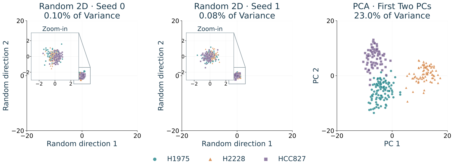
Two PCs reveal groups but retain only 23% of the variance

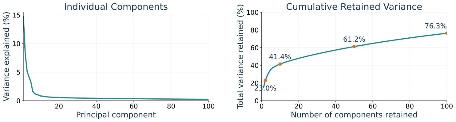
\[\text{Retained fraction}(k)=\frac{\sum_{j=1}^{k}\sigma_j^2}{\sum_{j=1}^{r}\sigma_j^2},\qquad r=\operatorname{rank}(X).\]

• Visualization: two coordinates already reveal cell-line structure.
• Reconstruction: 100 PCs retain 76.3%; reaching 90% requires 173 PCs.

[Sources] - source:scmixology-celseq2-counts-2019

All percentages refer to the same 274-by-2,000 centered, log-normalized matrix, not raw counts, all measured genes, or biological information. The denominator uses the full SVD spectrum, not just the first 100 components shown. Reducing 2,000 features to 100 retains 76.2775% of centered energy. The 90% threshold is an illustration, not a recommended universal rule. Components beyond 100 are computed but not plotted; the threshold occurs at 173. No new derivation. The small last singular value reflects centering; numerical residual energy is negligible. Ask how visualization and reconstruction lead to different k choices.

The same PCA plot supports different questions about usefulness

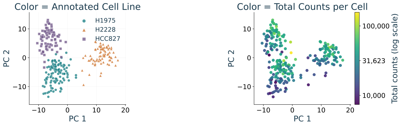
Discuss: Do these plots justify saying that PCA preserved the biology we care about?

• What does agreement with known cell-line labels support?
• What might total counts per cell explain—and what evidence would you want next?

[Sources] - source:scmixology-readme-2019 - source:scmixology-celseq2-counts-2019 - source:scmixology-celseq2-metadata-2019

Merged interpretation and evidence activity, about two minutes. These are the same coordinates, recolored after fitting. Left: labels supply an external annotation consistent with the visible groups; they did not train PCA. Right: total endogenous-gene counts before normalization vary across cells and still track some position within groups. Such counts can reflect both capture depth and biological RNA content. Color association alone does not establish a technical artifact or a biological cause, nor prove normalization has failed. We used one protocol, so this is not a claim about between-protocol batch effects. Seek known markers, independent measurements, replicate experiments, and a specified downstream purpose. Do not assume held-out evaluation terminology yet. The plot supports structure in this sample; it does not establish all relevant biology, disease prediction, a causal explanation, or future performance.

We fitted these observations; new cells need new evidence

From the original question…	…to what we established
Make thousands of measurements easier to inspect	Choose what the representation should preserve
Preserve observations under a squared-error criterion	PCA gives the best rank-\(k\) linear reconstruction
Compute that representation	Center, use SVD, and attend to finite precision
Inspect this cell dataset	Two PCs reveal known groups, but retain only 23% of variance

For new cells: keep the fitted preprocessing, gene set, mean, and directions fixed.

Before moving on: what general lessons does this case teach us about building useful representations?

[Sources] - source:scmixology-celseq2-counts-2019

The case wraps the arc: purpose, formalization, solution, numerical computation, and interpretation. New cells must use the same measurement definitions and preprocessing rule; reuse selected genes, fitted means, and PCA directions. This analysis used every cell for fitting and makes no held-out performance claim. The closing question opens the broader task of turning representations into useful predictions, discoveries, or decisions and evaluating those uses. Generalization is one part of that larger question, not the only destination. Do not start a train/test or classifier tutorial here. The following retrospective connects this case to the principles developed across the arc.

A useful solution begins with deciding what to preserve

Gene-expression measurements → desired representation → objective → constraints → solution

Choice we made	What it allowed us to specify
Which measurements, preprocessing, and units?	The observations and geometry
What should the representation preserve?	Squared reconstruction error
Which transformations are allowed?	A linear representation with \(k\) coordinates
What is the best solution under those choices?	Leading right singular vectors of centered data

Formalization makes a vague goal solvable. Choosing the goal remains our responsibility.

Arc-level synthesis, not a new derivation. Revisit the full chain from the original cell-data question. PCA’s optimality is conditional on the objective, representation, and constraints; it does not choose those for us.

Representations preserve some structure and discard other structure

In our cell-expression example	What it teaches us
Two PCs reveal known cell-line groups	A small representation can expose useful structure
Those two PCs retain only 23% of variance	Visible groups do not imply faithful reconstruction
100 PCs retain 76.3% of variance	The number of coordinates depends on the purpose

• Rank and discarded singular values describe linear information loss.
• Low-dimensional structure need not be linear: recall the curved-data example.
• Large variance is not automatically the variation that matters for our task.

Ask what was preserved, what was lost, and whether that matches the intended use.

[Sources] - source:scmixology-celseq2-counts-2019

Percentages refer to the same centered 274-by-2,000 log-normalized matrix used in the case. This summarizes the figures students just inspected. Distinguish linear reconstruction dimension from a useful two-coordinate visualization.

A proof, a working computation, and useful evidence are different achievements

Question	What this arc established
Did we solve the stated problem?	SVD gives the optimal linear PCA reconstruction
Did we compute it correctly and efficiently?	Shapes, broadcasting, operation order, and finite precision matter
Does the result accomplish our purpose?	Real-data evidence supports particular claims, with limits

A mathematical guarantee does not establish every practical claim we might want to make.

Next question: What evidence would justify trusting a learned rule on new observations?

Close Arc 2 before opening a predictor example in Arc 3. A correct numerical implementation can produce a representation that is not useful for a chosen purpose. A useful plot of fitted observations does not by itself establish performance for future observations. Do not teach train/validation/test here.

Binary Prediction: Goals and Historical Data

David I. Inouye

September 21, 2026

What would justify trusting a prediction for someone we have never seen?

Opening of Arc 3. This topic formalizes the goal before introducing historical training data or methods. The complete arc outline is tentative. This opening stops at the question that motivates KNN; do not teach evaluation procedures yet.

Different settings ask the same kind of prediction question

Setting	Information available	Question with two possible answers
Bank phone campaign	Customer attributes and prior contact history	Will this customer open a term-deposit account?
Wine screening	Chemical measurements such as acidity and alcohol	Will this wine receive a high sensory rating?
Activity recognition	Measurements from motion sensors	Is this person walking?

In each case, use available information to predict an outcome we do not yet know.

Our running case: will a customer open a term-deposit account—depositing money for a fixed period to earn interest?

[Sources] - source:uci-bank-marketing - source:uci-wine-quality - source:uci-smartphone-activity

These are three real dataset settings. The bank case uses UCI Bank Marketing, whose label describes taking up a term deposit, not a credit-card application. Explain the product before using the shorter phrase “open the account.” For the proposed wine binary task, define high rating as a sensory score >=7; this cutoff is our choice, not a universal commercial standard. For the sensor example, recode WALKING, WALKING_UPSTAIRS, and WALKING_DOWNSTAIRS as walking, and SITTING, STANDING, LAYING as not walking. State the recoding if asked. Original wine labels are ordinal and original HAR labels have six classes. At this stage the sensor question concerns an unknown current activity, not necessarily forecasting a future event. Inputs need not be images.

A useful prediction begins with a precise question

A bank calls customers to offer a term-deposit account: money deposited for a fixed period to earn interest.

Ask first	Our initial specification
Who is the prediction about?	A new customer in the population we intend to contact
When do we need the answer?	Before calling the customer
What may we use?	Information available at that moment
What outcome are we predicting?	Whether the customer opens the offered account during the campaign
What does “best” mean for now?	Make as few prediction mistakes as possible on new customers

How can we express that goal precisely enough to reason about it?

[Sources] - source:uci-bank-marketing

The source calls the outcome “subscribed a term deposit.” Use “opened the offered term-deposit account” as the plain-language explanation. This is the recorded campaign outcome, not necessarily the result of one call; campaigns may include multiple contacts. Do not invent a 30-day window. This predicts response, not the causal effect of calling. Equal mistake costs are the initial modeling choice.

Binary classification turns the question into inputs, outcomes, and a predictor

Object	Meaning in the bank case
\(\boldsymbol{x}\in\mathcal X\)	Customer information available before calling
\(y\in\{0,1\}\)	Actual outcome: did not open (0) or opened (1) the offered account
\(f:\mathcal X\to\{0,1\}\)	A rule that predicts an outcome from the available information
\(\widehat y=f(\boldsymbol{x})\)	Our prediction for this customer

\[ \boldsymbol{x}\quad\xrightarrow{\quad f\quad}\quad\widehat y\in\{0,1\}. \]

A prediction is correct when \(f(\boldsymbol{x})=y\). The same abstraction describes all three opening cases.

Which predictor would we want if we could choose the best one?

No training set or algorithm has been defined. Mathcal X denotes the space of valid representations; not every attribute must already be a numerical feature. We will decide how to encode the information when a method requires it. A rule returning 0 or 1 is not automatically a good rule.

The goal is minimum error on new customers

A distribution \(p\) describes how likely different customer–outcome pairs are. For a randomly selected customer, \(\boldsymbol{\mathrm X}\) is their information and \(\mathrm Y\) is what actually happens: these are random variables drawn jointly from \(p\).

Intuition: how likely is our prediction \(f(\boldsymbol{\mathrm X})\) to match \(\mathrm Y\)? We formalize the opposite event—the population error:

\[ R_p(f)=\Pr_{(\boldsymbol{\mathrm X},\mathrm Y)\sim p} \bigl(f(\boldsymbol{\mathrm X})\ne\mathrm Y\bigr). \]

Goal: choose \(f^*\in\operatorname*{arg\,min}_{f:\mathcal X\to\{0,1\}} R_p(f)\).

• Minimizing error is equivalent to maximizing accuracy, \(1-R_p(f)\).
• This specifies our goal; it does not yet tell us how to find or evaluate \(f\).

We know what we want. What information do we actually have?

p is the unknown joint distribution of inputs and outcomes, not a dataset or a known table. Explain probability in words before reading the equation. Argmin means a predictor attaining the smallest error; we are not deriving the Bayes classifier here. Do not assume the minimum is zero or that every outcome is fully determined by the available input. No empirical average or train/test split is introduced yet. The goal can be defined without assuming i.i.d. historical data; that assumption enters when using historical data to address it.

We have historical examples, not future answers

A real bank dataset records customer information and whether the customer opened the offered account.

Record	Age	Job	Housing loan?	Opened account?
1	56	Housemaid	No	No
3	37	Services	Yes	No
76	41	Blue-collar	Yes	Yes

Selected actual records from a term-deposit phone campaign; not a representative sample.

We call the labeled examples available for constructing a predictor the training data:

\[\mathcal D=\{(\boldsymbol{x}_i,y_i)\}_{i=1}^{n}.\]

When can outcomes for past customers tell us something about new customers?

[Sources] - source:uci-bank-marketing - source:uci-bank-marketing-data

Exact records 1, 3, and 76 (one-based, excluding header) from bank-additional/bank-additional-full.csv in the archived bank-additional.zip. The source y column is yes/no for taking up a term deposit. “Opened account?” is a plain-language rendering of that label, not a new target. Record 76 is the first positive example; the selection does not estimate prevalence. Record ID is not a feature; rows are not guaranteed unique customers. The version has 41,188 records. These are real measurements, not the superseded illustrative mail case.

Using the past requires a connection to the future

Working assumption: new customers resemble past customers in both their available information and how that information relates to opening the offered account.

Our clean mathematical model is i.i.d. sampling:

• Identically distributed: past and new input–outcome pairs come from the same \(p\).
• Independent: one sampled example does not supply information about another draw.
• The new case is independent of the historical sample used to construct \(f\).

Same distribution does not mean the same people or exactly repeated feature values.

Before using the historical table, will its inputs even be available at prediction time?

I.i.d. means independent and identically distributed. It is a working model, not an established fact about the bank dataset. Both features and conditional outcomes must match, not just similar account histories. Repeated customers and chronological changes can violate these assumptions; flag rather than analyze those now. A distribution p defines the target; i.i.d. is a separate assumption about sampled evidence. Local smoothness, introduced with KNN later, is yet another assumption and does not follow merely from i.i.d. sampling.