Binary Prediction: From the Goal to KNN

ECE 57000 — September 23, 2026

David I. Inouye

We will revisit the Arc 3 opening as a concise recap

We will go through the revised Arc 3 opening again, but more quickly this time.

The slides are unchanged from the new arc sequence. Because the ideas should now be review, we will focus on their connections and move faster through details.

This is an intentional exception to the usual recap pattern. Do not summarize the opening slides. Present them again in their complete revised sequence, but at review pace. Slow down only if the revised connections remain unclear.

Binary Prediction: Goals and Historical Data

David I. Inouye

Last updated: September 22, 2026

What would justify trusting a prediction for someone we have never seen?

Opening of Arc 3. This topic formalizes the goal before introducing historical training data or methods. The complete arc outline is tentative. This opening stops at the question that motivates KNN; do not teach evaluation procedures yet.

Different settings ask the same kind of prediction question

Setting	Prediction question with two possible answers
Bank phone campaign	Will this customer open a term-deposit account?
Wine screening	Will this wine receive a high sensory rating?
Activity recognition	Is this person walking?

Each uses information available now to predict an outcome we do not yet know.

Our running case: the bank phone campaign. A term-deposit account holds money for a fixed period to earn interest.

[Sources] - source:uci-bank-marketing - source:uci-wine-quality - source:uci-smartphone-activity

These are three real dataset settings. The bank case uses UCI Bank Marketing, whose label describes taking up a term deposit, not a credit-card application. Explain the product before using the shorter phrase “open the account.” For the proposed wine binary task, define high rating as a sensory score >=7; this cutoff is our choice, not a universal commercial standard. For the sensor example, recode WALKING, WALKING_UPSTAIRS, and WALKING_DOWNSTAIRS as walking, and SITTING, STANDING, LAYING as not walking. State the recoding if asked. Original wine labels are ordinal and original HAR labels have six classes. At this stage the sensor question concerns an unknown current activity, not necessarily forecasting a future event. Inputs need not be images.

Each practical question needs a mathematical counterpart

Practical question	Bank-case answer	Mathematical counterpart
What information is available?	New customer information known before the call	?
What answer do we want?	Whether the customer opens the offered account	?
What makes a predictor good?	Few mistakes across unseen customers	?

We will fill in one mathematical counterpart at a time.

[Sources] - source:uci-bank-marketing

The source calls the outcome “subscribed a term deposit.” Use “opened the offered term-deposit account” as the plain-language explanation. This is the recorded campaign outcome, not necessarily the result of one call; campaigns may include multiple contacts. Do not invent a 30-day window. This predicts response, not the causal effect of calling. Equal mistake costs are the initial modeling choice. Read the first two columns from left to right. The question marks create three specific gaps that the following slides fill in this same row order.

Available information becomes the input \(\boldsymbol{x}\)

Question: What information is available?

Bank-case answer: New customer information known before the call.

Formalization:

\[\boldsymbol{x}\in\mathcal X\]

\(\boldsymbol{x}\) is one customer’s available information; \(\mathcal X\) is the set of valid input representations.

This fills the first row of the opening map. Examples include age, job, and information from completed prior campaigns if known before the call. Not every attribute must already be numerical. We will decide how to encode information when a method requires it. Do not introduce the training dataset yet.

The desired answer becomes the output \(y\)

Question: What answer do we want?

Bank-case answer: Whether the customer opens the offered account.

Formalization:

\[ \boldsymbol{x} \quad\xrightarrow{\quad f\quad}\quad \widehat y\in\{0,1\} \]

\(y\in\{0,1\}\) is the actual outcome. The prediction is correct when \(\widehat y=y\).

This fills the second row of the opening map. The predictor f receives the available input and returns a predicted outcome. Keep prediction \(\widehat y\) distinct from actual outcome y. The actual outcome may be observed later, but the framework also covers outcomes that are already determined and merely unseen. No training process or algorithm has been defined.

Population error formalizes few mistakes on unseen customers

A distribution \(p\) describes how common different unseen customer–outcome pairs are. A random pair \((\mathbf{x},\textnormal{y})\) drawn from \(p\) contains the available information and what actually happens.

The population error is the chance that our prediction is wrong:

\[ R_p(f)=\Pr_{(\mathbf{x},\textnormal{y})\sim p} \bigl(f(\mathbf{x})\ne\textnormal{y}\bigr). \]

Goal: choose \(f^*\in\operatorname*{arg\,min}_{f:\mathcal X\to\{0,1\}} R_p(f)\).

This completes the goal—but it does not tell us how to find \(f\).

p is the unknown joint distribution of inputs and outcomes, not a dataset or a known table. Explain probability in words before reading the equation. Argmin means a predictor attaining the smallest error; we are not deriving the Bayes classifier here. Do not assume the minimum is zero or that every outcome is fully determined by the available input. No empirical average or train/test split is introduced yet. The goal can be defined without assuming i.i.d. historical data; that assumption enters when using historical data to address it.

The prediction contract now has a mathematical form

Practical question	Bank-case answer	Mathematical counterpart
What information is available?	New customer information known before the call	Input \(\boldsymbol{x}\in\mathcal X\)
What answer do we want?	Whether the customer opens the offered account	Outcome \(y\in\{0,1\}\); prediction \(\widehat y=f(\boldsymbol{x})\)
What makes a predictor good?	Few mistakes across unseen customers	Small population error \(R_p(f)\)

The unresolved question: How do we find the right function \(f\)?

Return to exactly the same map shown with question marks. Read the completed third column top to bottom and emphasize the unresolved question. This is the concise synthesis of the prediction contract, not a new inventory.

Machine learning infers the rule \(f\) from examples

In ordinary computation, the rule is given. For example, a circuit simulator is given equations and parameters, then computes an output from an input.

Ordinary computation

\[f\ \text{given},\qquad \boldsymbol{x}\longmapsto f(\boldsymbol{x})\]

Machine learning

\[\mathcal D=\{(\boldsymbol{x}_i,y_i)\}_{i=1}^{n} \quad\longmapsto\quad \text{infer } f\]

The historical input–outcome pairs \(\mathcal D\) are the training data. They give examples of the mapping, but not the rule itself.

[Sources] - source:uci-bank-marketing

This is the central conceptual hinge. Many conventional programs are supplied with a rule or procedure: a simulator is given governing equations and a sorting routine is given its ordering procedure. Machine learning instead receives example inputs paired with observed outputs and must construct a rule that also works for unseen inputs. Do not imply that the inferred rule is unique or that training examples alone guarantee success.

A dataset column is not automatically an allowed input

The real prediction context defines what each \(\boldsymbol{x}_i\) may contain.

Prediction moment: before calling this customer.

Historical column	Status at prediction time
Recorded age and job	Available before the call
Duration of this call	Unavailable until after the call
Whether the customer opens this account	The outcome \(y_i\), not an input

The dataset records each call’s duration after that call ends.

Can call duration be used to predict whether this customer will open the account before the call begins?

A. Yes, because it appears in the historical training data.

B. Yes, if the historical dataset is sufficiently large.

C. No, because it is unavailable at the prediction moment.

C. No. Training inputs must represent what would actually be known when the prediction is made; more records do not repair that mismatch.

Larger principle: available columns describe a dataset; allowed inputs are determined by the real decision we are trying to support.

[Sources] - source:uci-bank-marketing - source:uci-bank-marketing-data

This subtle distinction deserves emphasis but not a long detour. Pairs, about two minutes. Current call duration is a real dataset column, yet it is unavailable before calling. More records do not repair the mismatch. A completed prior campaign can be known before the present decision. Other fields need the same prediction-time audit. This is a problem-formulation issue, not merely a later data-cleaning step.

Assumptions mark where a learned predictor can break

Training pairs are the evidence. Performance on unseen pairs is the claim. An explicit assumption must connect them:

\[ \underbrace{\text{training pairs}}_{\text{observed evidence}} \quad\xrightarrow{\quad\text{assumption}\quad}\quad \underbrace{\text{unseen pairs}}_{\text{desired claim}} \]

The most common simple starting point is i.i.d. sampling: model the training pairs and unseen pairs as independent draws from the same distribution \(p\).

I.i.d. is deliberately naive. When it reasonably approximates the problem, it provides a useful foundation for analysis. We will use it for now.

Begin from the evidence-to-claim gap before unpacking the letters in i.i.d. Training data alone cannot establish how unseen cases behave. We must state the assumption that licenses the connection. I.i.d. is common because it is simple enough to analyze and often a useful first approximation, not because every real dataset satisfies it. The next two slides make its two parts explicit. Later sections revisit what changes when either part is implausible, including changes to the data unit, evaluation design, or target population.

Independence rules out linked training examples

The first “I” in i.i.d. is independent.

Knowing one sampled pair \((\mathbf{x}_i,\textnormal{y}_i)\) should not change the probability of another draw once the population distribution is fixed. The unseen case should also be independent of the sample used to construct \(f\).

Possible violation: if the same customer appears after several campaign contacts, those rows and outcomes may be linked rather than independent examples.

Start with independence because it is the first I. This is a modeling assumption, not an established fact about the bank dataset. The source states that campaigns may involve multiple contacts, but records are not guaranteed to be unique people; present the repeated-customer example as a possible violation, not a claim about the released rows. Clustered households or coordinated campaigns are other examples, but omit them unless discussion needs one.

Identically distributed connects training pairs to unseen cases

The second “I” in i.i.d. is identically distributed.

Training pairs and the unseen pairs we care about are modeled as draws from the same joint distribution \(p\)—both the inputs and how they relate to the outcome.

Possible violation: if the bank changes who it contacts or changes the offered account, deployment cases may no longer follow the training distribution.

Same distribution does not mean the same customers or repeated feature values.

State the working assumption in plain language: unseen customers resemble past customers in both their available information and how that information relates to opening the offered account. This is stronger than saying the input columns have the same names. A random split cannot establish that unseen deployment cases follow the same distribution.

The contract and evidence now motivate a first method

The contract asks for low error on unseen customers using only information available before the call. Training pairs become evidence under our working assumption that they and the unseen cases are connected.

First idea: find past customers similar to the new customer and consult their outcomes.

Next question: What should “similar” mean, and why should their outcomes help?

This is the transition into KNN, not yet its implementation or evaluation. The next draft will construct a first neighbor-based rule, explain local smoothness, and then ask how to measure its success. Do not imply that merely returning an answer achieves the population optimum or that the historical dataset supplies unseen outcomes directly.

2. How can examples produce a predictor?

KNN makes learning from local evidence visible without making the algorithm the point.

KNN predicts from nearby observed outcomes

For a new customer \(\boldsymbol{x}\):

1. compute the distance to every training input \(\boldsymbol{x}_i\);
2. keep the indices \(\mathcal N_k(\boldsymbol{x})\) of the \(k\) nearest;
3. average their observed outcomes and take a majority vote.

\[ \widehat\eta_k(\boldsymbol{x}) =\frac{1}{k}\sum_{i\in\mathcal N_k(\boldsymbol{x})}y_i, \qquad \widehat y=\mathbb 1\!\left[\widehat\eta_k(\boldsymbol{x})\geq\tfrac12\right]. \]

The method constructs a prediction directly from the stored examples.

Use a small odd value of k for the first verbal example. The average is a local positive fraction; the threshold turns that estimated probability into a binary prediction. Do not optimize k yet. The point is that a learning rule can be constructed from examples without fitting a parametric formula.

Changing the axes can change who is nearest

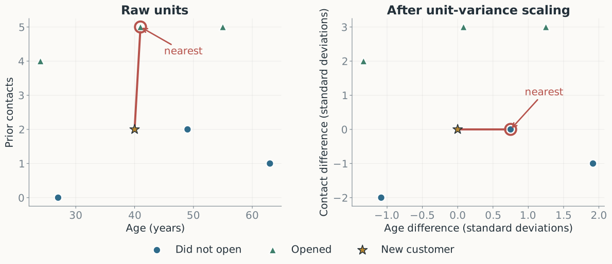
Distance measures differences in the coordinates we supply—not an intrinsic notion of customer similarity.

This is an illustrative bank-campaign example, not a claim about a particular row of the UCI data. The new customer is age 40 with two completed prior contacts. One historical customer differs by one year and three contacts; another differs by nine years and no contacts. Raw Euclidean distance privileges the age unit. After scaling age by 12 years and prior contacts by one contact, the neighbor flips. The plot is generated by lectures/scripts/arc3_knn_figures.py.

Unit-variance scaling is a simple default metric

For each feature \(j\), estimate its training mean and standard deviation, then use

\[ x'_{ij}=\frac{x_{ij}-\widehat\mu_j}{\widehat s_j}. \]

• Apply the same rule to numeric columns and binary indicator columns.
• Encode categorical attributes first—for example, with one indicator per category.
• Estimate \(\widehat\mu_j\) and \(\widehat s_j\) from training data only; remove constant columns.

Interpretation: every retained coordinate has empirical variance one before distance is computed.

This is the most natural baseline when no domain knowledge supplies feature weights. It does not prove that the resulting metric is meaningful. Never assign unordered categories arbitrary integers and then interpret numerical distance. For a binary indicator with prevalence p, the standard deviation is sqrt(p(1-p)); consequently a rare indicator receives a relatively large scaled difference. Mention this only as a reason to validate the metric, not as a new detour. Fit all preprocessing within the training split.

The neighbor fraction estimates a local outcome probability

The population quantity is

\[ \eta(\boldsymbol{x}) =\Pr(\textnormal{y}=1\mid\mathbf{x}=\boldsymbol{x}). \]

KNN substitutes nearby observed outcomes for repeated outcomes at exactly the same input:

\[ \widehat\eta_k(\boldsymbol{x}) =\frac{\text{nearby customers who opened the account}}{k}. \]

Similar customers need not have identical outcomes; their probabilities must be locally related.

The local fraction estimates eta, while the majority vote is the corresponding classification decision under equal mistake costs. Different labels among nearby customers can reflect information not represented in x rather than an algorithmic error. This creates the need for a local-smoothness argument.

With more data, \(k\) can grow while neighborhoods stay local

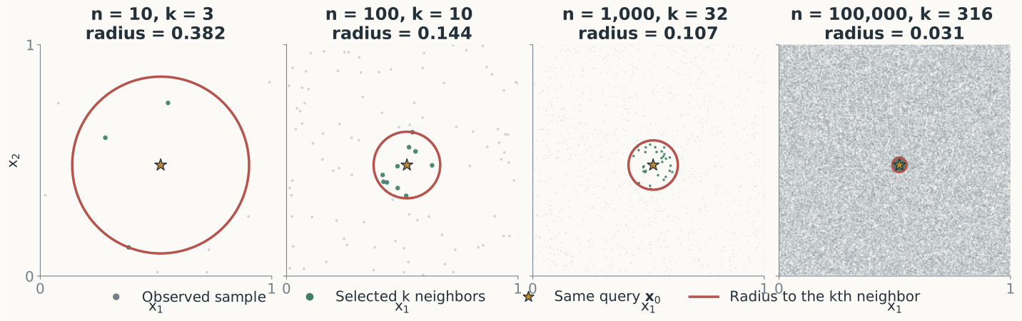
Here \(k=\lfloor\sqrt n\rfloor\), so \(k\to\infty\) while \(k/n\to0\): the same query averages more labels inside a smaller neighborhood.

[Sources] - source:stone-consistent-nonparametric-regression-1977

This is a controlled simulation with two abstract standardized coordinates, not an empirical bank result. Every panel uses the same query and a nested prefix of one sample sequence. Gray points are all observations, teal points are the k selected neighbors, and the red circle reaches the kth neighbor. The sqrt(n) schedule is illustrative: it satisfies the classic consistency direction but is not presented as universally optimal for a finite dataset. Increasing k reduces label noise; keeping k/n small allows the physical neighborhood to contract as the sample becomes dense. Stone’s result is much broader than this visualization; do not present a proof.

Smooth local structure is easier to estimate with finite data

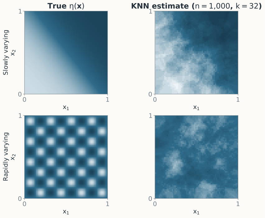
Local averaging recovers slowly varying probabilities sooner. Fine-scale or choppy structure can remain blurred until the sample is extraordinarily dense.

This is a finite-sample intuition, not an assertion that differentiability is required for every asymptotic consistency theorem. The lower response surface oscillates rapidly. With n=1,000 and k=32, each neighborhood averages across several changes in probability. The figure is generated by the same deterministic script as the growing-data illustration.

KNN defers nearly all computation until prediction

def fit(X, y):
    return np.asarray(X, float), np.asarray(y)

def predict_proba(model, X_new, k):
    X, y = model
    d2 = ((X_new[:, None, :] - X[None, :, :])**2).sum(2)
    nbr = np.argpartition(d2, k - 1, axis=1)[:, :k]
    return y[nbr].mean(axis=1)

Fit

• no parameter optimization
• store \(n\times d\) inputs and \(n\) labels
• memory and copy: \(O(nd)\)

Predict one input

• compute all \(n\) distances
• partial selection avoids a full sort
• time: \(O(nd)\)

Small reference sets can be cheap; very large ones motivate models that compress training evidence into learned parameters.

This is intentionally one efficient illustrative implementation, not a survey of trees, approximate search, batching, or production libraries. np.argpartition avoids sorting all n distances. A fully vectorized batch materializes a queries-by-training matrix, so large applications batch the queries. Say that fit has no optimization, not literally zero work: data still must be validated, transformed, and stored. Preview parametric linear and deep models without teaching them here. The dimensionality problem returns near the end of the arc.

3. Why can fitting the examples mislead us?

Observed success may reflect memorization, sample luck, or the wrong flexibility.

Which \(k\) looks best when we score the data used to fit it?

Assume every recorded input is distinct. We fit each KNN model, then compute its error on those same examples.

Which value of \(k\) should we select using only this error estimate?

A. \(k=1\)

B. \(k=15\)

C. \(k=151\)

A. \(k=1\). Every training example is its own nearest neighbor, so this procedure reports zero error.

That makes \(k=1\) look perfect—but our goal concerns unseen customers.

Live multiple choice, about two minutes. Poll before revealing. The best answer under the stated procedure is A, not because it necessarily generalizes best, but because scoring the fitted sample rewards memorization. Distinct inputs avoid the edge case of identical feature vectors with conflicting labels. This should create the need for a different source of evaluation evidence.

Training error answers an easier question

Quantity	Examples being scored	Question answered
Training error	Used to construct \(f\)	How well does \(f\) reproduce evidence it already saw?
Population error \(R_p(f)\)	Unseen draws from \(p\)	How often will \(f\) fail on the cases we care about?

The same observations cannot simultaneously serve as unrestricted construction material and untouched evidence of generalization.

Return to the population objective from the opening. The problem is not that training error is computed incorrectly; it answers a different, easier question. KNN makes the mismatch especially visible, but the distinction applies to every learned predictor.

A holdout lets observed data play the role of unseen data

We do not have outcomes for the genuinely unseen customers we ultimately care about. How can we estimate their error?

\[ \underbrace{\mathcal D_{\mathrm{train}}}_{\text{construct }f} \qquad\Big|\qquad \underbrace{\mathcal D_{\mathrm{holdout}}}_{\text{pretend unseen; score once}} \]

Reserve some observed pairs before fitting. Because their outcomes did not help construct \(f\), predictions on them mimic the information boundary of an unseen case—under the same sampling assumptions.

Lead with the question, pause briefly, then give the simple answer: act as though some observed examples are unseen by withholding them during training. The connection is informational, not temporal; the holdout may consist of historical rows. This is a development holdout at this stage, not yet a final test set. The i.i.d. assumption is what connects its errors to the target population.