Why Fitting Examples Can Mislead Us

ECE 57000 — September 25, 2026

David I. Inouye

Wednesday connected prediction goals, local evidence, and evaluation

• We defined the prediction contract using only information available when the prediction is made.
• Under an explicit i.i.d. working assumption, KNN uses nearby historical outcomes to estimate a local outcome probability.
• Training error scores evidence the predictor already used; a holdout creates untouched evidence that can stand in for unseen cases.

Today: use held-out evidence to understand how model flexibility, data, and representation affect prediction on unseen cases.

Keep the title, recap, and repeated Wednesday stopping slide to five minutes combined. Reconnect the ideas rather than reteaching the earlier slides.

September 25 pacing plan (50 minutes, including an eight-minute reserve): - Slides 1–3: title, recap, and Wednesday stopping slide, 5 minutes. - Slides 4–5: cross-validation mechanics and flexibility, 6 minutes (11 elapsed). - Slides 6–8: bias, the real-data illustration, and the error identity, 11 minutes (22 elapsed). - Slides 9–10: the two key derivations, 10–12 minutes (32–34 elapsed). - Slide 11: average over inputs, 4 minutes (36–38 elapsed). - Slides 12–13: k tradeoff and data/representation synthesis, 4 minutes (40–42 elapsed).

Expected stop: slide 13, completing the bias–variance argument before Question 4. If the derivations or discussion run long, slide 11 is a coherent fallback stop; do not rush the cross-term reasoning to reach the two synthesis slides. If slide 13 ends before about minute 40, the six ready runway slides open Question 4. A two-to-three-slide extension reaches its training-error check and validation solution. Only start the 4.5% selection question with time for the answer and explanation. The full runway ends with train/validation/test roles; it is prepared capacity, not an additional requirement for this meeting. The later cross-validation, refitting, and evaluation-boundary slides remain in the standalone topic deck for the next class.

A holdout lets observed data play the role of unseen data

We do not have outcomes for the genuinely unseen customers we ultimately care about. How can we estimate their error?

\[ \underbrace{\mathcal D_{\mathrm{train}}}_{\text{construct }f} \qquad\Big|\qquad \underbrace{\mathcal D_{\mathrm{holdout}}}_{\text{pretend unseen; score once}} \]

Reserve some observed pairs before fitting. Because their outcomes did not help construct \(f\), predictions on them mimic the information boundary of an unseen case—under the same sampling assumptions.

Repeat Wednesday’s stopping slide briefly for continuity. The connection is informational, not temporal; the holdout may consist of historical rows. This is a development holdout at this stage, not yet a final test set. The i.i.d. assumption connects its errors to the target population.

Cross-validation rotates which fold is held out

Split one observed dataset into folds. Each fold takes one turn as untouched evaluation data.

	Fold 1	Fold 2	Fold 3	Fold 4	Fold 5
Fit 1	score \(e_1\)	train	train	train	train
Fit 2	train	score \(e_2\)	train	train	train
Fit 3	train	train	score \(e_3\)	train	train
Fit 4	train	train	train	score \(e_4\)	train
Fit 5	train	train	train	train	score \(e_5\)

\(K\) fits produce \(K\) errors, then we average: \(\widehat R_{\mathrm{CV}}=\frac1K\sum_{j=1}^{K}e_j\)

Leave-one-out cross-validation is the small-data extreme: \(K=n\).

The five-column bar is one dataset, not five separately collected datasets. Five or ten folds are common, but do not present either as universally best. Fit scaling and every learned preprocessing step inside each training fold. The fold errors are correlated because the training sets overlap, so CV does not create K independent experiments. CV is less central in many modern large-data workflows, but students should know the term and computational structure. About three minutes.

The neighbor count controls how much local detail survives

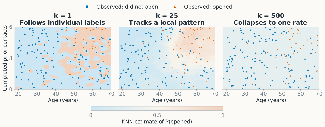
\(k=1\) can overfit individual outcomes; using every example erases useful local structure. Held-out error can reveal both failures.

This slide begins the flexibility question after cross-validation completes the held-out-evaluation idea. The illustration uses a controlled response simulation with plausible bank-case coordinates, not an empirical result from the UCI Bank Marketing data. Small k preserves sample noise, intermediate k borrows local evidence, and k=n underfits by returning the global positive rate everywhere. Do not claim that k=25 is optimal outside this illustration.

Bias compares the average fitted estimate with the target relationship

At one fixed test point \(\boldsymbol{x}\), imagine refitting the method on many possible training samples. Their average prediction is where the method tends to land:

\[ \mu(\boldsymbol{x}) =\mathbb E_{\mathcal D}\!\left[\widehat\eta_{\mathcal D}(\boldsymbol{x})\right], \qquad \operatorname{Bias}(\boldsymbol{x}) =\mu(\boldsymbol{x})-\eta(\boldsymbol{x}). \]

Real data lets us observe how estimates vary across samples. It does not reveal the true \(\eta(\boldsymbol{x})\), so formal bias remains unknown.

Bias is a property of a learning procedure across possible training samples, not merely one fitted model’s visible error. Keep the discussion at one fixed test point. Real observations do not reveal eta, so the later empirical figure can illustrate sample sensitivity but cannot measure formal bias.

Bias measures offset; variance measures spread

At age 40 (the only feature), each blue dot uses a different disjoint training set \(\mathcal D\) of \(n=1{,}647\) or \(1{,}648\) records. Each row reuses the same 25 sets.

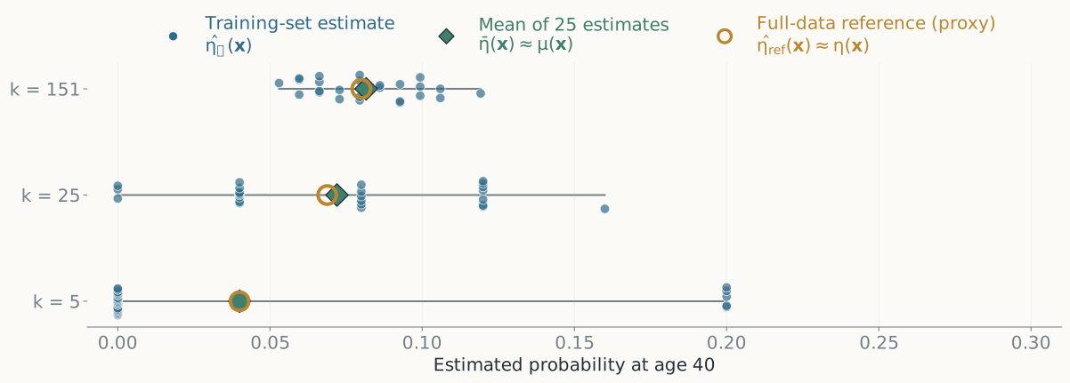
\[ \operatorname{Bias}(\boldsymbol{x}) ={\color{#3f7f6b}\mu(\boldsymbol{x})} -{\color{#b8872f}\eta(\boldsymbol{x})} \]

\[ \operatorname{Var}_{\mathcal D}\!\left({\color{#2f6b8a}\widehat\eta_{\mathcal D}(\boldsymbol{x})}\right) =\mathbb E_{\mathcal D}\!\left[ \left({\color{#2f6b8a}\widehat\eta_{\mathcal D}(\boldsymbol{x})} -{\color{#3f7f6b}\mu(\boldsymbol{x})}\right)^2\right] \]

True \(\eta\) is unknown: the diamond-to-ring gap is a bias proxy. The reference may itself be biased.

[Sources] - source:uci-bank-marketing-data

The 41,188 archived bank records are randomly partitioned into 25 disjoint training datasets: 13 contain 1,648 records and 12 contain 1,647. Each fit trains on one subset, unlike cross-validation, which trains on the complement of a held-out fold. All three rows reuse the same subsets and the same fixed query, age 40, with age as the only feature. Within each subset, the estimate averages the outcomes of its k nearest neighbors; n is the training-set size, not k. Diamonds mark the mean of the 25 estimates, an empirical approximation to mu. Gold rings are full-data reference fits using approximately the same neighbor fraction (25k neighbors). Neither marker is the unknown true eta. The empirical spread illustrates the theoretical variance over possible training samples; the finite partition does not measure that population quantity exactly. The diamond-to-ring difference is only an illustrative bias proxy. Because the reference uses the same neighbor fraction, it can share the small-sample fits’ smoothing bias. A small gap therefore does not establish small true bias. The approximation to eta in the legend is a working proxy, not a verified claim of accuracy. The equations define population bias and variance; the plotted mean and spread approximate their corresponding expectations over training samples. Vertical offsets only separate dots for readability. Discrete stacks occur because each estimate is an average of binary labels. A wider neighborhood may increase bias even when it reduces sample sensitivity.

Expected squared error combines bias, variance, and label noise

Draw a new input \(\mathbf{x}\) and binary outcome \(\textnormal{y}\) from the target population, independently of the training set \(\mathcal D\). How far is the predicted probability from the actual outcome, averaged over new cases and refits?

\[ \begin{gathered} \underbrace{\mathbb E_{\mathcal D,\mathbf{x},\textnormal{y}} \left[(\widehat\eta_{\mathcal D}(\mathbf{x})-\textnormal{y})^2\right]} _{\text{expected squared prediction error}} \\[0.6em] =\mathbb E_{\mathbf{x}}\!\left[ \underbrace{\operatorname{Bias}(\mathbf{x})^2}_{\text{systematic mismatch}} + \underbrace{\operatorname{Var}_{\mathcal D}(\widehat\eta_{\mathcal D}(\mathbf{x}))}_{\text{sample sensitivity}} + \underbrace{\eta(\mathbf{x})(1-\eta(\mathbf{x}))}_{\text{unresolved outcome variation}} \right]. \end{gathered} \]

Squared error loss gives this exact sum. Modeling choices can trade bias against variance; the represented inputs determine the remaining outcome noise.

This is squared error for probability estimation, not a decomposition of 0-1 classification error or accuracy. Explain the three terms intuitively before the following slides derive the identity by first conditioning on a fixed input and then averaging over the input distribution. Both x and y are random here; their joint distribution allows y to depend on x. Only the new pair is independent of the training dataset. Keep the label-noise term subordinate: the main instructional contrast is systematic mismatch versus sensitivity to the sampled training data.

Centering the outcome at \(\eta\) separates estimation error and noise

Fix \(\boldsymbol{x}\). Write \(\widehat\eta_{\mathcal D}=\widehat\eta_{\mathcal D}(\boldsymbol{x})\) and \(\eta=\mathbb E[\textnormal{y}\mid\boldsymbol{x}]\). The new outcome is independent of the training set given this input.

\(\displaystyle \mathbb E_{\mathcal D,\textnormal{y}}[(\widehat\eta_{\mathcal D}-\textnormal{y})^2\mid\boldsymbol{x}]\)

\(=\)

\(\displaystyle \mathbb E_{\mathcal D,\textnormal{y}}[((\widehat\eta_{\mathcal D}-\eta)+(\eta-\textnormal{y}))^2\mid\boldsymbol{x}]\)

(Add and subtract \(\eta\))

\(=\)

\(\displaystyle \begin{aligned}[t]&\mathbb E_{\mathcal D}[(\widehat\eta_{\mathcal D}-\eta)^2]+\mathbb E_{\textnormal{y}}[(\eta-\textnormal{y})^2\mid\boldsymbol{x}]\\&\quad+2\mathbb E_{\mathcal D}[\widehat\eta_{\mathcal D}-\eta]\,\underbrace{\mathbb E_{\textnormal{y}}[\eta-\textnormal{y}\mid\boldsymbol{x}]}_{\eta-\mathbb E[\textnormal{y}\mid\boldsymbol{x}]=\eta-\eta=0}\end{aligned}\)

(Expand; independence factors the cross term, and centering makes it zero)

\(=\)

\(\displaystyle \mathbb E_{\mathcal D}[(\widehat\eta_{\mathcal D}-\eta)^2]+\underbrace{\mathbb E[\textnormal{y}^2\mid\boldsymbol{x}]-\eta^2}_{\operatorname{Var}(\textnormal{y}\mid\boldsymbol{x})}\)

(Expand the remaining outcome square)

\(=\)

\(\displaystyle \underbrace{\mathbb E_{\mathcal D}[(\widehat\eta_{\mathcal D}-\eta)^2]}_{\text{probability-estimation error}}+\underbrace{\eta(1-\eta)}_{\text{outcome noise}}\)

(Binary \(\textnormal{y}^2=\textnormal{y}\), so \(\eta-\eta^2=\eta(1-\eta)\))

The starting expression is squared prediction error against a new outcome at a fixed input. Each subsequent equality is one reveal; the expanded square and its zero cross term appear together. Conditional independence of the new outcome and D factors that cross term. Its outcome factor is zero because eta is the conditional mean. Expanding the remaining outcome square gives E[y squared | x] - 2 eta E[y | x] + eta squared, hence E[y squared | x] - eta squared. For a binary outcome, y squared equals y. Conditioning on bold italic x abbreviates random bold upright x equals this fixed input. D-only expectations need no conditioning bar because the new input and training dataset are independent. Every fit is still evaluated at this x. This intermediate expression separates error in estimating the probability from outcome noise; the next slide decomposes the estimation error. Allow five to six minutes, including student questions about the cross term.

Centering the fit at \(\mu\) separates squared bias and variance

At the same fixed \(\boldsymbol{x}\), let \(\mu=\mathbb E_{\mathcal D}[\widehat\eta_{\mathcal D}]\). Continue from the preceding slide, keeping its outcome-noise term.

\(\displaystyle \mathbb E_{\mathcal D}[(\widehat\eta_{\mathcal D}-\eta)^2]+\eta(1-\eta)\)

\(=\)

\(\displaystyle \mathbb E_{\mathcal D}[((\widehat\eta_{\mathcal D}-\mu)+(\mu-\eta))^2]+\eta(1-\eta)\)

(Add and subtract \(\mu\))

\(=\)

\(\displaystyle \begin{aligned}[t]&\mathbb E_{\mathcal D}[(\widehat\eta_{\mathcal D}-\mu)^2]+(\mu-\eta)^2+\eta(1-\eta)\\&\quad+2(\mu-\eta)\,\underbrace{\mathbb E_{\mathcal D}[\widehat\eta_{\mathcal D}-\mu]}_{\mathbb E_{\mathcal D}[\widehat\eta_{\mathcal D}]-\mu=\mu-\mu=0}\end{aligned}\)

(Expand; \(\mu-\eta\) is constant across training sets, and the centered fit has mean zero)

\(=\)

\(\displaystyle \underbrace{(\mu-\eta)^2}_{\text{squared bias}}+\underbrace{\mathbb E_{\mathcal D}[(\widehat\eta_{\mathcal D}-\mu)^2]}_{\text{variance}}+\underbrace{\eta(1-\eta)}_{\text{outcome noise}}\)

(The cross term is zero; reorder the remaining terms)

This exact sum uses squared error loss. Other losses need different analyses.

Continue the same equality chain from the preceding slide. The expanded square and the explanation of its zero cross term are one reveal, not a later aside. Mu and eta depend on the fixed input but do not vary across D, so pull mu minus eta outside the expectation. The remaining factor is zero by the definition of mu. No independence between hat_eta_D and its own deviation is assumed. Bias is where the procedure tends to land relative to the true probability; variance is how much it moves when its training sample changes. Noise remains even at the true probability. The learning procedure and sample size are fixed across refits. The next slide averages the pointwise identity over inputs to recover the population formula. Allow five to six minutes, including discussion of why mu minus eta is constant across training datasets.

Averaging over inputs gives population squared prediction error

Now draw a new input \(\mathbf{x}\) from the target population and its outcome \(\textnormal{y}\). Average the pointwise identity over those inputs:

\[ \begin{gathered} \underbrace{\mathbb E_{\mathcal D,\mathbf{x},\textnormal{y}} [(\widehat\eta_{\mathcal D}(\mathbf{x})-\textnormal{y})^2]}_{\text{average error on new cases, across refits}} \\[0.6em] =\underbrace{\mathbb E_{\mathbf{x}}[\operatorname{Bias}(\mathbf{x})^2]}_{\text{average squared bias}} +\underbrace{\mathbb E_{\mathbf{x}}[\operatorname{Var}_{\mathcal D}(\widehat\eta_{\mathcal D}(\mathbf{x}))]}_{\text{average variance}} +\underbrace{\mathbb E_{\mathbf{x}}[\eta(\mathbf{x})(1-\eta(\mathbf{x}))]}_{\text{average outcome noise}}. \end{gathered} \]

• Inputs count according to how often they occur in the target population. The decomposition stays exact, but its terms now summarize all inputs.
• Average squared bias: positive and negative biases at different inputs cannot cancel each other.

Why it matters: smoothing can reduce sample sensitivity while increasing systematic mismatch. Held-out error measures their combined effect, plus outcome noise.

The left-hand side averages over both hypothetical refits and independent new test cases. It describes the learning procedure at a fixed sample size, rather than the risk of one particular fitted model. For one realized dataset D, test risk averages only over x and y; the displayed decomposition holds after also averaging over D. For probability estimation against eta instead of a realized outcome, omit the noise term on both the pointwise and population versions. Linearity of expectation preserves the three-term sum without extra cross terms. E_x[Bias(x)^2] is not (E_x[Bias(x)])^2. Local failures can still be hidden by a population average, particularly for rare inputs. The noise is unresolved given the represented inputs, not necessarily irreducible under richer features. Real held-out labels estimate total prediction error, not these separate unknown components. This explains why knowing that k reduces variance does not by itself tell us which k gives the best predictions. About three minutes.

Increasing \(k\) exchanges local detail for stability

Smaller \(k\)	Larger \(k\)
uses closer evidence	reaches farther from the query
follows more sample-specific detail	averages more observed outcomes
often lower local bias, higher variance	often higher local bias, lower variance

Neither extreme is automatically best. Held-out error measures the combined effect for the population and representation we care about.

Use “often” deliberately. Actual bias, variance, and classification error need not change monotonically with k. Reconnect the table to the flexibility figure and the real-data sampling variation rather than introducing a generic U-shaped cartoon as fact.

Data and representation improve the same local-evidence mechanism

Change	What happens to a KNN neighborhood?
More representative training data	genuinely similar examples can be closer
Better scaling or features	distance favors differences relevant to the outcome
Larger \(k\)	more outcomes are averaged, but evidence comes from farther away

All three change the evidence inside \(\widehat\eta_k(\boldsymbol{x})\) and therefore its bias and variance.

This synthesis closes Question 3. More data does not automatically help if it comes from the wrong population, and better representation does not remove the need for evaluation. The next question asks how held-out evidence changes once we use it to choose among alternatives.

4. How can we choose a model without fooling ourselves?

Choosing a predictor and measuring its performance are two different uses of data.

Which neighbor count should we choose?

We fit KNN with \(k=1,5,25\) and choose the lowest training error. Inputs are distinct, and each training point counts as its own neighbor.

Is this a reliable way to choose the best predictor for new cases?

A. Yes: evaluating every candidate on the same examples makes the comparison fair.

B. No: training error rewards reproducing outcomes the predictor already used.

C. No: we should always choose the largest \(k\) to get the most stable predictions.

B. Here, \(k=1\) gets zero training error by retrieving each point’s own label. That does not establish how well it predicts a new outcome.

Live retrieval check, about two minutes. The setup ensures the self-neighbor argument is exact, avoiding conflicting labels at duplicate inputs. Same-data comparison does not fix the reuse of training labels. C confuses stability with overall prediction quality: excessive smoothing can introduce bias. Reconnect to the earlier training-versus-population error distinction before introducing validation as the appropriate evidence for choosing k.

A held-out validation set lets us compare candidate values of \(k\)

Fit each candidate using \(\mathcal D_{\mathrm{train}}\). Evaluate its predictions on the same separate \(\mathcal D_{\mathrm{validation}}\), then choose the lowest validation error.

\[ \mathcal D_{\mathrm{train}} \xrightarrow{\ \text{fit}\ } f_1,f_5,f_{25} \xrightarrow{\ \text{score on validation}\ } \widehat k=\arg\min_{k\in\{1,5,25\}}\widehat R_{\mathrm{validation}}(f_k). \]

The validation outcomes are unavailable when fitting each candidate. They give us evidence about prediction on cases outside that candidate’s training set.

About two minutes. Validation is the appropriate role for choosing k. Candidates and their preprocessing are fitted using training data only. Under independent, representative sampling, each fixed candidate’s empirical validation error is unbiased for its population error. This does not make either the winning score or the selection decision “unbiased”; choosing the best true model remains uncertain with finite data. Defer that distinction to the next question. The errors in this section are 0–1 classification errors, not the squared probability errors used in the preceding bias–variance identity.

What does the selected model’s 4.5% error tell us?

We choose \(k\) with the lowest validation error and report its 4.5% as the selected model’s estimated population error.

Across repetitions of this procedure, is the reported error lower on average, unbiased, or higher on average?

A. Lower than the selected model’s true population error on average.

B. Unbiased for the selected model’s true population error.

C. Higher than the selected model’s true population error on average.

A: optimistic selection bias. Choosing the lowest observed error also favors favorable validation noise. Validation appropriately helps choose \(k\), but the winning score is no longer an unbiased final evaluation.

Live multiple choice, about three minutes. The 4.5% is an illustrative scenario, not a measured result from the bank dataset. Compare each selected model’s validation error with that same model’s true population error, then average over repetitions. Fixed candidates may each have unbiased validation scores, yet choosing the minimum introduces downward selection bias. Correlations among candidate scores and the number of choices affect its magnitude. The bias can be zero in degenerate cases; never claim that every observed validation error must be below its population error. A particular selected model may truly have population error below 4.5%. Nor is selecting k guaranteed to find the population optimum. The method is appropriate for selection, while reuse of its winning score as a final estimate creates the problem. Error optimism corresponds to accuracy optimism in the opposite direction: 4.5% error is 95.5% accuracy.

Validation is held out of each fit, but participates in selection

What are we evaluating?	Did validation outcomes help construct it?
One candidate fitted at a fixed \(k\)	No: only the training data determined that fit.
The selected pipeline, including the choice of \(k\)	Yes: validation errors determined which candidate won.

Selection is part of learning. Information from validation enters through our choice of \(k\), even though the KNN fitting step never reads those labels.

The same reuse occurs when validation guides features, preprocessing, or model families. It leaks into a claimed final evaluation through those choices.

About three minutes. This is indirect information reuse, distinct from scoring on the very rows used for fitting. It can be much subtler than training-set reuse, but do not promise it is always small: extensive adaptive searching can severely overfit validation data. Using validation to select is intentional and appropriate; treating its selected score as untouched final evidence is the mistake. Human error inspection and AI-driven iteration also belong to the selection process when they influence the final pipeline. For this reason the information boundary must surround the full process, not just model.fit().

Separate validation for choosing from test data for reporting

Reserve all three roles before development:

Data	Role	What may it influence?
Training	Fit each candidate.	Its learned parameters or stored examples.
Validation	Compare candidates and choose \(k\).	The selected pipeline.
Test	Score the settled pipeline once.	The reported performance estimate.

Freeze the pipeline before using the test outcomes. An independent, representative test set gives an unbiased error estimate for that fixed pipeline, with finite-sample uncertainty.

About three minutes. If refitting on training plus validation data after selecting k, complete that refit before opening the test set; the test evaluates that refitted predictor. Fit any learned preprocessing within the permitted fitting data. Do not change the pipeline in response to test performance and retain the same claim of untouched evaluation. Cross-validation can rotate the validation role within development data, but a final independent test role is still needed for an honest final estimate after selection. This slide resolves both earlier questions: training fits, validation chooses, and test evaluates the result of the whole development process. An unbiased estimate can still be noisy or unrepresentative of deployment if the sampling assumptions fail.