Choosing Models and Evaluating the Whole Pipeline

ECE 57000 — September 28, 2026

David I. Inouye

Friday connected model flexibility and trustworthy evaluation

• At a fixed input, squared prediction error separates into squared bias, training-sample variance, and unresolved outcome noise.
• Changing \(k\), available data, or representation changes which nearby evidence the model uses.
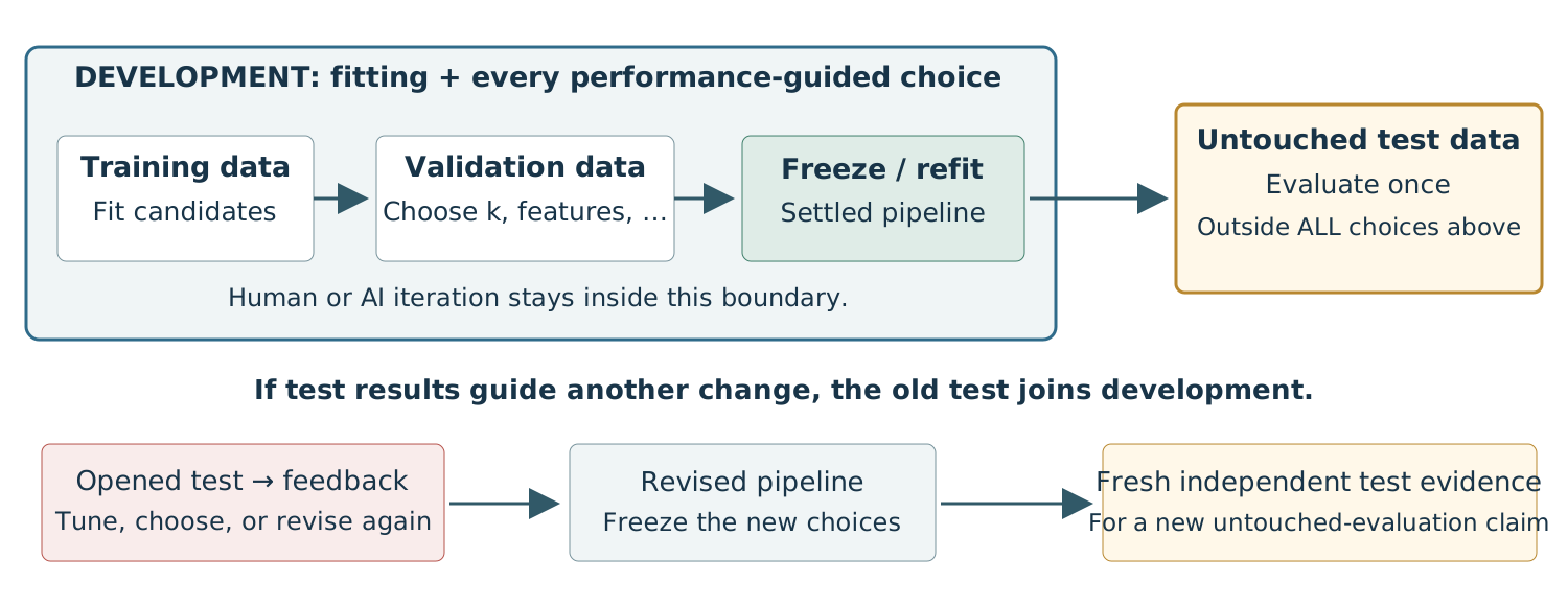
• Validation chooses a pipeline; its winning score is optimistic on average. Final test data must stay outside the entire selection process.

Today: finish the development/evaluation boundary, then examine how finite and imperfectly matched evidence limits our claims.

September 28: use the calibrated 0.8 timing factor and keep five minutes of reserve. With the previous stopping slide restored, the main prefix is about 42 minutes and the full deck about 52 minutes; expect to reach some runway if discussion is brief. Aim to finish the controlled bank noise experiment; the bounded evaluation claim is a natural earlier stop if discussion runs long. Five fully authored runway slides explain noisy distance, connect real review data to a learned 1D score and Arc 4. Allow roughly 10–12 minutes for that continuation if reached. Question 5 follows measurement → deployment relevance → supported claim, with a rough 95% interval and a sample-size table, with no PAC/concentration formalism. The two .quick-poll questions are brief commitment-and-reveal checks. CV was already covered; this continuation uses a simple train/validation/test split.

Separate validation for choosing from test data for reporting

Reserve all three roles before development:

Data	Role	What may it influence?
Training	Fit each candidate.	Its learned parameters or stored examples.
Validation	Compare candidates and choose \(k\).	The selected pipeline.
Test	Score the settled pipeline once.	The reported performance estimate.

Freeze the pipeline before using the test outcomes. An independent, representative test set gives an unbiased error estimate for that fixed pipeline, with finite-sample uncertainty.

This is where the previous class ended. Briefly reestablish the three roles before introducing refitting. Training fits, validation chooses, and test evaluates the result of the whole development process. Fit learned preprocessing within the permitted fitting data. If refitting on training plus validation after selection, complete that refit before opening the test set; the test evaluates that refitted predictor. An unbiased estimate can still be noisy or fail to represent deployment.

Refit the chosen pipeline before opening the test set

After choosing \(k\) and all other pipeline settings, we may fit once more on training + validation data to use all development examples.

\[ \underbrace{\mathcal D_{\mathrm{train}}\cup\mathcal D_{\mathrm{validation}}}_{\text{refit with settled choices}} \quad\longrightarrow\quad f_{\mathrm{final}} \quad\xrightarrow{\ \mathcal D_{\mathrm{test}}\ }\quad \widehat R_{\mathrm{test}}(f_{\mathrm{final}}). \]

For KNN, this means storing all development examples with the chosen \(k\) and refitting any learned preprocessing on those development examples.

The test result describes this final predictor. Changing it after seeing the test result turns that test into more development evidence.

About three minutes. Refit is optional, but the order matters. More development examples can change the learned predictor even when its settings stay fixed. Thus the earlier winning validation score does not directly score the refitted predictor. The untouched test set does. Decide the refitting procedure before opening the test set. This does not guarantee that refitting always improves performance or that the k selected on smaller fits remains optimal. If test results motivate further changes, acknowledge renewed development and obtain fresh independent evidence before making another untouched-evaluation claim.

Keep final testing outside every development feedback loop

One final test can cover all development choices. A new split is needed when we reuse final-test feedback to make further choices—not for every fitting step.

About two minutes. This makes the information boundary visible. The test must remain outside preprocessing, hyperparameter selection, feature decisions, and human or AI error-driven iteration. Independent representative testing gives an unbiased estimate for the fixed evaluated pipeline; it does not remove sampling uncertainty or population mismatch. Merely observing a test score does not force a new split if the model remains fixed. Reusing its outcomes to select a revision does change its role. CV remains in the previously delivered introductory slide; this continuation uses only train/validation/test. Next: what can the resulting score tell us about real deployment?

5. When and why should a learned solution hold?

A test score becomes useful when we understand its uncertainty and the scope of its evidence.

Interpret the score through three connected questions

Our reasoning process	Question to resolve
1. What did the test measure? ← now	How much evidence is behind this score?
2. Does it represent deployment?	Could dependence, population, or available information differ?
3. What can we claim?	State the supported result and the conditions for extending it.

We protected the test from selection. Now interpret what it tells us.

Brief orientation. No PAC-style guarantee unit here. The point is to distinguish an honest but finite measurement from a claim about future deployment.

A rough 95% interval is the score ± two standard errors

Fix the model before testing on \(m\) independent examples from the target population. Let \(\widehat a\) be the fraction of test predictions that are correct.

\[ \text{Approximate 95\% interval:}\qquad \widehat a\ \pm\ 2\sqrt{\frac{\widehat a(1-\widehat a)}{m}}. \]

900 correct out of 1,000: 90% accuracy, with a margin of about 1.9 percentage points.

“With approximately 95% confidence, this fixed model’s accuracy in this population is between 88% and 92%.”

About two minutes. [Sources] source:nist-binomial-confidence-intervals. Accuracy is an average of independent Bernoulli correct/incorrect indicators. Its estimated standard error is sqrt(a_hat(1-a_hat)/m); 1.96 is the usual normal 95% multiplier, rounded to 2. At 900/1000 the two-standard-error margin is 1.897 percentage points, so the displayed whole-percent sentence is deliberately rough. If repeated independent test samples were used to build these intervals, roughly 95% would cover the fixed population accuracy under the approximation. This is not a 95% probability for each prediction or a guarantee for a new population. A common rough adequacy check is at least ten correct and ten incorrect outcomes; near 0%/100% or at small m, use Wilson (examples in notes), not a zero-width Wald interval. This formula is for ordinary accuracy or binary error rate, not directly for balanced accuracy, F1, AUC, subgroup comparisons, or dependent windows. No PAC learning statement or epsilon/delta formalism. Hold the model and population fixed.

A rough normal approximation: use Wilson intervals for small samples or few errors. This measures finite-test uncertainty, not protection against leakage or distribution shift.

More test examples support more precise claims

Suppose measured accuracy is 90% in each case:

Independent test examples	Correct predictions	Rough 95% margin (pp)
10	9/10 = 90%	±19†
30	27/30 = 90%	±11†
100	90/100 = 90%	±6
1,000	900/1,000 = 90%	±1.9
2,000	1,800/2,000 = 90%	±1.3
5,000	4,500/5,000 = 90%	±0.8
10,000	9,000/10,000 = 90%	±0.6

10–30: wide uncertainty. 1,000–10,000: roughly 2-point to sub-1-point precision here.

About two minutes. [Sources] source:nist-binomial-confidence-intervals. Displayed margins are 100 × 2sqrt(.9 × .1 / m), rounded: 18.97, 10.95, 6.00, 1.90, 1.34, 0.85, 0.60 percentage points (m=10,30,100,1000,2000,5000,10000). These are normal-approximation scales, not Wilson half-widths. At m=10 or 30 there are too few errors for reliable normal coverage; the dagger explicitly marks those rows. Do not interpret 90% ±19 points as a valid interval or simply clip it at 100%. For actual small-sample intervals, Wilson gives 59.6%–98.2% for 9/10 and 74.4%–96.5% for 27/30 (z=1.959963984540054). For m=10, even nine correct predictions supports only about 60%–98% accuracy. At 1000 the interval is about 88.0%–91.7%; at 10000 about 89.4%–90.6%. Margin shrinks like 1/sqrt(m): ten times more precision needs 100 times more data. Emphasize practical percentage-point precision rather than decimal-place targets. Report the estimate with its margin and decide whether that precision is useful. For rare failures, subgroup scores, or high-stakes decisions, even 10000 may be insufficient. More same-population data cannot repair deployment mismatch.

pp = percentage points. Margins use the previous slide’s rough formula. †Small-sample scale only: use Wilson for an actual interval. Fixed model; independent, representative test examples.

Next ask whether the evidence matches deployment

Our reasoning process	What we have established
1. What did the test measure?	A count of errors from a finite sample.
2. Does it represent deployment? ← now	Check independence, population, and available information.
3. What can we claim?	Combine the measured result with the scope of its evidence.

A very large test set can measure the wrong deployment population very precisely.

About 30 seconds. Numbers are not meaningless when an assumption fails. Identify which inference needs that assumption and what weaker claim remains. This section traces assumptions to concrete failure modes and evaluation choices.

Repeated rows need not provide independent evidence

Imagine 100 customers, each represented by 10 related campaign records.

• A random row split may put the same customer in both training and test data.
• A model may exploit person-specific information that will not help on a new customer.
• The 1,000 rows also need not provide the precision of 1,000 independent customers.

If the claim concerns new customers, keep each customer in one split.

About two minutes. Hypothetical example, not a claim that UCI has verified customer IDs or precisely this duplication. Dependence does not necessarily bias every sample mean, but treating the rows as independent understates uncertainty. Effective sample size depends on dependence structure; do not declare it exactly 100. Shuffling rows does not make related observations independent. If deployment is future events for known people, the relevant design can differ.

Independent examples can still come from a different population

\[ R_p(f)=\Pr_{(\mathbf{x},\textnormal{y})\sim p}\{f(\mathbf{x})\ne\textnormal{y}\}, \qquad R_q(f)=\Pr_{(\mathbf{x},\textnormal{y})\sim q}\{f(\mathbf{x})\ne\textnormal{y}\}. \]

• The test set estimates performance under \(p\).
• Deployment may draw customers and outcomes from \(q\ne p\): distribution shift.
• Out-of-distribution (OOD) performance depends on \(q\); even perfect knowledge of \(R_p(f)\) does not determine \(R_q(f)\).

What changes operationally—and could it change who responds to our offer?

About two minutes. This breaks the identical-distribution link between evaluation and deployment even if each sample separately consists of independent examples. OOD here means a changed joint distribution, not necessarily feature values outside the observed range. Shift can change performance mildly, severely, or not at all; its effect depends on the model and the changed relationship.

Would this new contact list preserve accuracy?

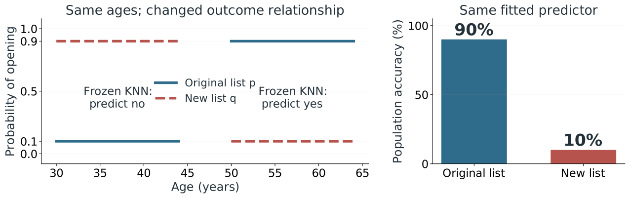
Synthetic bank campaign: a frozen age-only KNN model is 90% accurate under the original list. A new supplier provides the same age distribution and same overall account-opening rate.

Do those checks establish similar accuracy on the new list?

A. Yes: the input distribution and overall outcome rate are unchanged.

B. No: the relationship between age and opening may have changed.

C. Yes, if we make the original-list test set much larger.

B. Matching the separate summaries does not establish a matching joint relationship.

About two minutes, one commitment and reveal. This is a deliberately constructed synthetic case; no empirical UCI result or typical effect size is claimed. The new supplier is operationally ordinary, not mathematically a small change. C tightens estimation of the old population instead of measuring the new one.

The unchanged predictor falls from 90% to 10% accuracy

Synthetic bank example. Both lists: half ages 30–44, half ages 50–64; uniform ages within each group; 50% open overall. Only the relationship between age and outcome changes.

The old 90% remains valid for the old population. More old-list data cannot establish new-list accuracy.

About two minutes. Generated by lectures/scripts/arc3_shift_figure.py. Train once on 3,000 controlled source examples: 100 at each integer age, exactly 10% opening at each younger age and 90% at each older age. Fix k=101 and age as the only input; majority vote yields no for every younger age and yes for every older age. The generator evaluates exact population risks over 30 equally likely ages, not a tuned lucky test sample. Conditional probabilities reverse under q, so accuracy reverses exactly. The balanced 50% outcome rate is for clarity and is not the real bank dataset prevalence. The q outcomes are never used in fitting. A possible mechanism is a different mix of unobserved savings preferences within each age group. This is a hypothetical story, not a causal discovery: matching p(x) and p(y) does not establish matching p(x,y). No new age values are needed. The source-population result stays meaningful. Additional source test samples reduce sampling uncertainty, not the deployment gap. If useful at the board, write Rhat_p-R_q=(Rhat_p-R_p)+(R_p-R_q); the identity stays in notes rather than requiring another slide. This deliberately severe shift is not claimed typical.

Which test matches the claim about new people?

A walking classifier uses many sensor windows from each volunteer. Deployment will involve people absent from development data.

Which split most directly tests that claim?

A. Randomly assign windows to training and test sets.

B. Put each volunteer entirely in development or entirely in test.

C. Test later windows from volunteers already used for training.

B. It tests unseen people. It still does not establish transfer to different sensors, activities, or collection settings.

About two minutes. A transfer question using the smartphone-activity setting, source:uci-smartphone-activity. This is a hypothetical evaluation choice, not a new empirical result. A and C can support different claims about known people. Repeated windows within a test person remain correlated; grouping prevents person overlap but does not turn windows into independent people.

Choose the evaluation design from the deployment claim

Intended claim	More relevant evidence	What still needs reasoning?
More cases from the same population	Random held-out examples	Does the sample represent deployment?
Future campaigns	Train earlier, test on a later campaign	Will later changes resemble this one?
New customers	Keep each customer entirely in one split	Are these customers representative?

All designs require prediction-time inputs: current-call duration remains unavailable before the call. A split cannot repair that information mismatch.

About two minutes. No universally best split. Specify prediction unit, time, information, and intended population before choosing the design. Historical contacted clients do not automatically represent all potential customers. Chronological evaluation tests one observed transition, not every future shift. Changing a pipeline after inspecting a new-supplier test makes that data part of development; fresh final evidence is then needed for an untouched claim.

Finally state what the evidence supports

Our reasoning process	What we have established
1. What did the test measure?	Report the errors and number of test examples.
2. Does it represent deployment?	Examine dependence, changed populations, and available inputs.
3. What can we claim? ← now	State the supported result and the conditions for extending it.

A useful number comes with a reasoned account of where it applies.

Brief orientation, about 30 seconds. Return to the same three-stage roadmap. The next slide turns this framework into a concrete report with scope and uncertainty.

Report a result, its scope, and its uncertainty

Illustrative report: “The frozen before-call predictor made 100 errors on 1,000 independent held-out customers from supplier A’s campaign: 10% error.”

• Scope: one prediction per customer; account opening as the outcome; test data excluded from all development choices.
• Uncertainty: roughly 10% ±1.9 percentage points at 95% confidence.
• Extension: a different supplier may change response patterns within age groups. This result does not establish its error without evidence connecting the populations.

Say what may change, why it matters, and what evidence would resolve it.

About two minutes. These are hypothetical report counts, separate from the exact population-risk calculation in the shift illustration. The outcome and metric must also match the business goal; accuracy alone does not establish profit or causal benefit. More precise measurement for p is not a substitute for evaluating relevance to q.

From interpreting evidence to rethinking the predictor

So far: What does a settled model’s test score tell us about deployment?

Now: When does KNN’s notion of “nearby” stop being useful—and what should we learn instead?

Our next steps:

1. See how near and far distances become less distinct in high dimensions.
2. Test what happens when irrelevant features distort distance.
3. Motivate a learned score that emphasizes predictive information.

Brief section transition, about 30 seconds. Close Question 5’s interpretation argument explicitly. We now change the modeling question: even with trustworthy evaluation, raw locality can be a poor basis for prediction. This is the bridge from Arc 3 to Arc 4, not another evaluation caveat or an OOD-method discussion. The train/validation/test boundary still applies when comparing predictors.

In high dimensions, near and far become less distinct

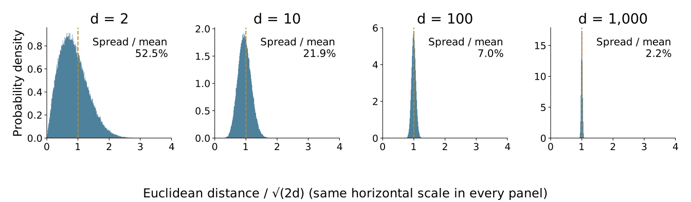
Draw 500 points with independent standard-normal coordinates: \(\mathbf{x}_i\sim\mathcal N(\boldsymbol{0},\mathbf I_d)\). Plot every pairwise distance.

Typical raw distance grows like \(\sqrt{2d}\); its relative spread shrinks. Dividing by \(\sqrt{2d}\) lets us compare dimensions on the same scale.

A “near” point is only slightly closer than a “far” point: distance loses contrast.

About two minutes. [Sources] source:cornell-cs4780-knn-2018. The older illustration used independent uniform coordinates in a unit cube. This is a new reproducible Gaussian simulation, generated by lectures/scripts/arc3_distance_concentration.py. Use 500 points and nested independent coordinates at d=2,10,100,1000, seed20260928. All 124750 unordered pairs are shown, not just neighbors or distance to the origin. Pairwise distances share observations and are not independent replicates. All horizontal axes and histogram bin widths match; vertical density scales vary so each distribution’s width remains legible. The dashed line marks one. Spread means standard deviation; the reported coefficient of variation is unchanged by normalization. Normalizing every distance by the same dimension-dependent number does not change the neighbor ranking. For two independent standard Gaussian vectors, squared distance / 2 has a chi-square law with d degrees of freedom: squared distance has mean 2d and variance 8d. Thus distance / sqrt(2d) concentrates near one. Raw Euclidean distance’s absolute standard deviation approaches one; it does not shrink to zero. Avoid saying all points have exactly equal distances, or using central quantiles as nearest/farthest extremes. With a fixed finite sample, relative near/far contrast shrinks as d grows; very different sample-size growth or structured data can change the conclusion. This motivates the bank noise experiment; concentration alone does not prove classification must fail for every high-dimensional distribution or metric. The complementary sparse-coverage argument: a uniform-cube box of side r holds fraction r^d; holding r fixed requires exponentially many samples for fixed occupancy.

Add measurements that contain no new information

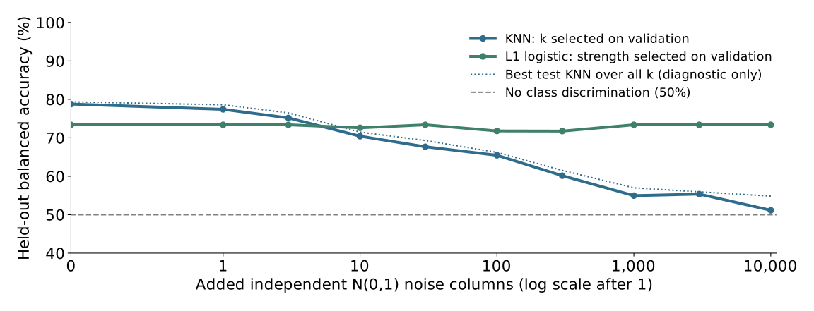
Return to our simulated bank campaign: age and prior contacts predict opening. Keep every customer and outcome fixed; append independent Gaussian columns.

\[ \boldsymbol{x}_{\mathrm{aug}}= [\,\text{age},\ \text{prior contacts},\ z_1,\ldots,z_d\,], \qquad \textnormal{z}_j\overset{\mathrm{iid}}{\sim}\mathcal N(0,1). \]

• Noise is independent of both the original features and the outcome.
• Standardize using training data; select \(k\) or regularization on validation.
• Same split: 500 training, 500 validation, 2,000 test customers.

Available predictive information is unchanged. Is distance still useful?

About two minutes. This is the original bank_flexibility simulation, not measured UCI bank data. Its nonlinear response law and seed 572 are unchanged. Append nested columns from one independent Gaussian draw with seed 20260928. Both methods get identical standardized features and class-balanced decisions. Every feasible k=1..500 is considered; L1 logistic C is selected from .001,.003,.01,.03,.1,.3,1. No split/seed search. The linear model is deliberately misspecified for the nonlinear bank law and need not beat KNN without noise.

Independent noise can make neighbors nearly uninformative

Balanced accuracy: average of the two class recall rates; 50% means no discrimination. At 10,000 noise columns: KNN 51.1%; learned-score model 73.4% (preview of Arc 4).

About two minutes. Generated by lectures/scripts/arc3_bank_noise.py, with exact results in bank-noise-results.json. Balanced accuracy prevents majority-class prediction from hiding failure in this imbalanced case. KNN uses a class-balanced vote (opening fraction greater than training opening prevalence); logistic uses balanced class weights. Both tune on validation balanced accuracy. The dotted curve is the diagnostic maximum test score across every feasible k, not a valid selection procedure: even that reaches only 54.8% with 10,000 noise columns. One fixed experiment, not an average over random repetitions or a universal rate. The endpoints are 78.8% to 51.1% KNN and 73.4% to 73.4% logistic. Regularization suppresses many noise coefficients; unregularized linear fitting is not promised this stability. The nonlinear response law explains the lower linear baseline.

Noise dominates distance; which coordinates should matter?

\[ \|\boldsymbol{x}_{\mathrm{aug}}-\boldsymbol{x}'_{\mathrm{aug}}\|^2 =\underbrace{\|\boldsymbol{x}_{\mathrm{signal}}-\boldsymbol{x}'_{\mathrm{signal}}\|^2}_{\text{two relevant coordinates}} +\underbrace{\sum_{j=1}^{d}(z_j-z'_j)^2}_{\text{many irrelevant coordinates}}. \]

• Independent noise differences accumulate and scramble which customers are nearest.
• Increasing \(k\) averages more labels; it does not identify the relevant coordinates.
• Could we learn which coordinates matter, giving irrelevant ones less influence?

High dimension alone is not the verdict: correlated features can carry redundant, useful structure. Real data need not fill the whole ambient space.

About two minutes. Linear models have not yet been taught. Pose learned feature importance as the next idea; do not assume knowledge of linear scores or penalties. Before finite-sample standardization, two independent standard normal vectors contribute a noise sum with mean 2d and standard deviation sqrt(8d). Relative distances concentrate, while absolute nuisance fluctuations grow and can overwhelm bounded signal differences. Raw Euclidean KNN gives all standardized coordinates equal weight. This experiment demonstrates that failure mechanism, not a theorem that every metric or representation must fail. Sparse regularization uses supervised evidence; with more noise and insufficient data it too can fail. The next real example tests the nuance. Correlation or lower intrinsic dimension can help, but neither guarantees a good distance nor is measured for this corpus.

Real-world example: movie-review sentiment

• 2,000 real reviews: predict positive or negative sentiment.
• 18,746 vocabulary words: represent each review with one numerical feature per word.
• Shared words need not mean shared sentiment: “good” versus “not good.”

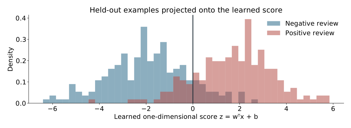
A new idea: learn a positive or negative score for each word and combine the contributions. This leads to a linear model, which we will study next.

About one minute. [Sources] source:cornell-movie-review-polarity-v2 and source:cornell-movie-review-polarity-v2-data. This is an introduction and motivation, not a lesson on linear models or text preprocessing. Do not discuss TF–IDF here. Distinguish the review’s numerical word features from the word contributions a supervised model will learn. The exact representation and comparison protocol remain documented in the next slide’s notes and the reproducible script. “Good” and “not good” are instructor-created phrases, not corpus quotations. They illustrate that lexical overlap is not sentiment equivalence. Do not imply that independent word scores fully resolve negation or word order; the measured unigram model also has those limitations. A learned score is a promising change of predictor, not a solution to every language phenomenon. Real text has structure; high ambient dimension alone does not force chance-level KNN performance.

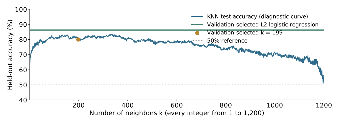
On real reviews, a learned score outperforms every tested \(k\)

Cornell movie reviews: positive versus negative sentiment; 18,746 word features. Train: 1,200 reviews; validate: 400; test: 400. No synthetic examples or added noise.

Validation-selected test accuracy: KNN 80.0%; learned word-score model 86.25%. Meaningful word features are not independent noise: KNN still has useful predictive signal.

About two minutes. The logistic regression curve previews the model family we will teach next; students need not know its training rule yet. Sources: source:cornell-movie-review-polarity-v2 and source:cornell-movie-review-polarity-v2-data. Original polarity v2.0, Pang and Lee, 2004. Fixed supplied filename folds cv0–5 train, cv6–7 validation, cv8–9 test; each split is class balanced. No split or seed search. Training-only unigram TF–IDF with min_df=2, sublinear_tf=True, norm=l2. Identical representation for both methods. KNN uses Euclidean distance, every k=1..1200, ties to negative; validation chooses k=199. L2 logistic selects C=100 from .01,.1,1,10,100 on validation. The test curve is diagnostic; test outcomes do not select hyperparameters. Correct counts are 320/400 versus 345/400; diagnostic best KNN is 334/400. This one split does not establish statistical superiority for all samples or prove dimensionality alone caused the gap. Labels derive from extracted ratings; the README warns unrecognized rating mentions can remain. This is within-corpus document evaluation, not author/movie/time-disjoint generalization or a guarantee for modern user reviews. Do not describe it as catastrophic KNN failure.

A useful one-dimensional projection separates the outcomes

\[ \boldsymbol{x}\in\mathbb R^{18746} \quad\longrightarrow\quad z=\boldsymbol{w}^{\mathsf T}\boldsymbol{x}+b\in\mathbb R \quad\longrightarrow\quad \widehat y=\mathbf 1\{z\ge0\}. \]

The weights are learned from training reviews; these distributions show held-out reviews.

About two minutes. The displayed x uses training-fitted TF–IDF; w and b were fit only on training examples, with regularization chosen on validation. The test labels color the diagnostic distributions but did not choose the projection or zero threshold. Histograms normalize within each class. A one-dimensional score does not mean all 18,746-dimensional inputs lie on a line.

Next: learn the predictive direction from labels

KNN asks which stored examples are nearby. A linear model learns how much each input contributes to one predictive score.

PCA preserves input variation; our goal is to separate outcomes.

Arc 4: How do labels tell us which weights to learn—and what can a linear score miss?

About one minute. Consolidate the PCA contrast and model-family handoff here. The score/projection visual has already introduced w^T x+b; do not repeat the classifier formula or preview an optimization syllabus. Linear models have not yet been taught. Next arc introduces the objective, fitting, and regularization. PCA/SVD is not a measured baseline for these reviews; do not claim it never helps. A predictive scalar score need not imply a one-dimensional input manifold. This is a different family of predictors f, not merely another value of k. All development/evaluation boundaries still apply to the learned direction.