Linear Regression, Logistic Classification, and the Definition of Convexity

ECE 57000 — October 2, 2026

David I. Inouye

Wednesday solved the linear regression fitting problem

• Ames sale prices gave us interpretable inputs and a numerical outcome.
• Squared residuals led to closed-form OLS through the normal equations.
• Residual orthogonality showed that no coefficient change can reduce training error.

Today: what does that solution mean, and what changes for classification?

September 30 ended at the fully revealed global-minimum proof (original PDF slide 29), with the projection illustration explicitly skipped. Recap in about one minute; repeat the exact stopping proof briefly, then continue to the training-error question. Keep the skipped projection illustration out of this meeting: the instructor deferred it because its explanation was not yet clear. The recording covered regression only, after about four minutes of exam discussion. Progress is ahead of the tentative calendar and modestly beyond the previous expected stop. Continue in the arc’s regression → classification → convexity → numerical optimization order. The expected stop targets the convexity guarantees; the prepared runway begins numerical optimization and develops regularization, local derivatives, step sizes, sampling, and Adam. The logistic probability-residual derivative remains in the standalone optimization topic for the next meeting. Do not reteach the complete OLS algebra. Keep this October 2 composition private until separately requested for release.

Orthogonality proves that no other fit has lower error

• \(\boldsymbol{r}=[r_1,\ldots,r_n]^{\mathsf T}\in\mathbb{R}^n\): one residual per observation, \(r_i=y_i-\widehat y_i\).
• \(\boldsymbol{r}\) has \(n\) coordinates for observations, not \(d\) coordinates for features like \(\boldsymbol{x}_i\).
• Recall OLS orthogonality: \(\widetilde X^{\mathsf T}\boldsymbol{r}=\boldsymbol{0}\); \(\boldsymbol{r}\) is perpendicular to each \(n\)-dimensional feature column.

Any other coefficient vector is \(\widehat{\boldsymbol{\theta}}+\boldsymbol{\delta}\); its prediction change \(\widetilde X\boldsymbol{\delta}\in\mathbb{R}^n\).

\(\displaystyle \|\boldsymbol{y}-\widetilde X(\widehat{\boldsymbol{\theta}}+\boldsymbol{\delta})\|^2\)

\(=\)

\(\displaystyle \|\boldsymbol{r}-\widetilde X\boldsymbol{\delta}\|^2\)

(Write the new residual)

\(\displaystyle \,\)

\(=\)

\(\displaystyle \|\boldsymbol{r}\|^2+\|\widetilde X\boldsymbol{\delta}\|^2\)

(\(\boldsymbol{r}^{\mathsf T}(\widetilde X\boldsymbol{\delta})=0\))

\(\displaystyle \,\)

\(\ge\)

\(\displaystyle \|\boldsymbol{r}\|^2\)

(A squared norm is nonnegative)

The bound is attained: choose \(\boldsymbol{\delta}=\boldsymbol{0}\), so \(\|\widetilde X\boldsymbol{\delta}\|^2=0\).

Thus \(\widehat{\boldsymbol{\theta}}\) achieves the smallest possible squared error, \(\|\boldsymbol{r}\|^2\): it is a global minimum.

Before the algebra, distinguish the spaces: n indexes observations (houses), d indexes features of one house. Both the stacked predictions and residuals have n coordinates. A feature column of the design matrix also has n coordinates, so its orthogonality with residuals is a dot product across observations, not across features. Here n=1758 training houses and d=226 encoded inputs; theta and delta have d+1 coordinates including the intercept. Zero delta is always optimal; it is the only optimal delta when the design has independent columns. Otherwise any delta in the null space also attains the bound, anticipating the redundancy slide. The omitted cross term is -2 r^T Xtilde delta = -2 (Xtilde^T r)^T delta=0. Reveal that justification with the second equality, not later. This establishes global optimality without assuming convexity already taught.

Does zero training residual alignment imply perfect prediction?

The OLS solution satisfies \(\widetilde X^{\mathsf T}\boldsymbol{r}=\boldsymbol{0}\).

Which conclusion follows?

A. Every residual is zero.

B. No linear coefficient adjustment reduces the training squared error.

C. The model will have zero error on future houses.

B. A nonzero residual can be perpendicular to the entire prediction subspace.

Two minutes. Transfer the projection geometry to distinguish optimality from interpolation and generalization. A vector can be nonzero yet orthogonal to every feature column. No test-data inference follows from the normal equations.

Redundant features can give the same fit with different coefficients

Example: predict a venue’s booking price from its room capacities (zero offset).

Feature	Seats	Model A coefficient	Model B coefficient
Room 1: \(x_1\)	20	1	0
Room 2: \(x_2\)	30	2	1
Total: \(x_3=x_1+x_2\)	50	0	1

\[\widehat y_A=1(20)+2(30)+0(50)=80,\qquad \widehat y_B=0(20)+1(30)+1(50)=80.\]

Same for every venue: \(x_2+x_3=x_1+2x_2\) whenever \(x_3=x_1+x_2\).

The data cannot distinguish these coefficient choices.

The inverse formula requires independent columns; redundant columns make \(\widetilde X^{\mathsf T}\widetilde X\) singular.

The room capacities, coefficients (dollars per seat), and booking prices are invented for arithmetic; no empirical booking-price claim. Both models use zero offset. Their weight difference is (-1,-1,1), whose dot product with every valid input is zero because total capacity is the sum of the two rooms. This is exact structural redundancy, not merely high correlation or a coincidence for the 20/30 example. Least squares still has a solution: remove redundancy or use an SVD-based solver. Individual coefficients need care; predictions are uniquely determined on the represented subspace. source:ames-housing-data. Full encoded Ames training matrix has centered rank219 versus226 features. The numerical comparison uses SVD least squares, not an invalid inverse. Fitted training responses are unique; test responses can differ for dependencies that do not persist. Do not turn this into a long numerical-analysis detour.

On real Ames sales, ordinary least squares is competitive

Same split: 1,758 train / 586 validation / 586 test; 226 encoded coordinates.

Model	Test RMSE ↓
Predict the training mean	$78,500
Validation-selected KNN	$32,800
Ordinary least squares	$26,300
Random forest	$25,700
Boosted trees	$25,200

A compact linear rule is useful here even alongside flexible nonlinear methods.

source:ames-housing-data; source:ames-housing-documentation. Fixed seed570, no test selection or outlier removal, train-only preprocessing. Tree methods are empirical reference points, not new methods taught here. One split supports competitiveness here, not universal superiority. RMSE is not a typical absolute-error guarantee; OLS MAE16400.

Held-out predictions reveal both useful structure and remaining errors

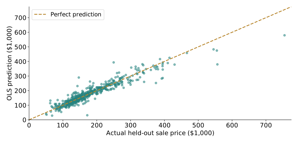
Each dot is one of 586 test sales. The diagonal means prediction equals outcome.

source:ames-housing-data. Full 226-coordinate OLS model, same fixed test split as the table. This is neither the one-input line nor training-fit evidence. Large expensive-house misses remain; aggregate error does not guarantee uniform accuracy across prices. Scope is historical Ames sales with this representation and split.

Solving the training problem leaves the prediction claim to evaluate

We can now explain: the function, the squared-error objective, the exact solution, and its geometry.

An exact fit to the objective does not make the model exact about the world.

Next: keep the linear score, but change from house prices to class probabilities.

30 seconds. Natural first-meeting boundary. Preserve train/validation/test as an established principle without repeating its full derivation.

From a solved fit to a fitting algorithm

Stage	Question
1. Interpret the OLS solution	What does the exact fit establish?
2. Choose a classification model and loss	How should a score predict and fit labels?
3. Understand the objective’s shape	When is a local optimum globally best?
4. Compute the coefficients	How can local information guide updates?

30 seconds. Stage 2 of the same four-stage roadmap. Name what the preceding stage established and the question this stage resolves. This guide is orientation, not a new derivation.

Classification changes what the score must predict

Regression: a numerical price, \(\widehat y=\boldsymbol{w}^{\mathsf T}\boldsymbol{x}+b\).

Classification: a positive/negative review, with an estimated class probability.

Return to our real Cornell case: 18,746 word features, 1,200 training reviews.

source:cornell-movie-review-polarity-v2; source:cornell-movie-review-polarity-v2-data. Thirty-second orientation; the case was motivated in Arc3.

Logistic regression follows model → objective → solution

1. Model — now: turn the score into a probability.

2. Objective — next: measure how well those probabilities predict the labels.

3. Solution — afterward: learn the coefficients by numerical optimization.

Thirty-second section divider after motivating the return to classification. Orient students to the same model–objective–solution progression used for linear regression; optimization is developed later.

A learned score combines signed contributions

For one review, let \(\boldsymbol{x}\in\mathbb R^d\) contain its word features.

\[ z=\boldsymbol{w}^{\mathsf T}\boldsymbol{x}+b =\sum_{j=1}^d w_jx_j+b. \]

• \(x_j\): the review’s measured feature; given at prediction time.
• \(w_j\): how that feature contributes; learned from labeled reviews.
• \(b\): a learned offset; \(z\): the resulting scalar score.

With \(d=18{,}746\), the model learns 18,747 parameters, not one parameter per review.

Three minutes. The corpus and feature count are from source:cornell-movie-review-polarity-v2 and source:cornell-movie-review-polarity-v2-data. Do not teach TF–IDF here. Distinguish observed x, learned w and b, and computed z. A scalar output need not imply that the input distribution lies on a line. Formally this score is affine when b is nonzero; “linear model” is the usual family name. Parameters are shared across all examples.

Each contribution is a weight times a measurement

Illustrative two-feature review, with invented weights:

Feature	Measurement \(x_j\)	Weight \(w_j\)	Contribution \(w_jx_j\)
“engaging”	2	\(+0.8\)	\(+1.6\)
“dull”	1	\(-1.1\)	\(-1.1\)
Offset	—	\(b=-0.2\)	\(-0.2\)

\[z=1.6-1.1-0.2=0.3\quad\Longrightarrow\quad\widehat y=1.\]

The model combines evidence; a word’s contribution depends on both its value and its weight.

Two minutes. These are invented counts and coefficients for arithmetic, not estimated coefficients from the review experiment. Use the zero threshold previewed last time; the next slide gives its geometry. Positive is label 1. The additive word representation does not model negation or word order.

A zero threshold divides space with a hyperplane

\[ \widehat y=\mathbf1\{\boldsymbol{w}^{\mathsf T}\boldsymbol{x}+b\ge0\}, \qquad \text{boundary: }\boldsymbol{w}^{\mathsf T}\boldsymbol{x}+b=0. \]

• In two dimensions, the boundary is a line; in three, a plane.
• \(\boldsymbol{w}\) determines its orientation; \(b\) shifts its position.
• Moving in a direction orthogonal to \(\boldsymbol{w}\) leaves the score unchanged.

Learning chooses which direction matters for the labels, rather than which examples are nearby in every coordinate.

Three minutes. Draw a two-dimensional line and its normal. For w nonzero, adding v with w^T v=0 preserves z. The score is a scaled projection plus an offset, not necessarily an orthogonal coordinate because w need not be a unit vector. PCA chose a direction for input variation; our objective will use outcomes.

A sigmoid converts the score into a probability estimate

\[ \widehat\eta(\boldsymbol{x})=\sigma(z)=\frac{1}{1+e^{-z}}, \qquad z=\boldsymbol{w}^{\mathsf T}\boldsymbol{x}+b. \]

Score \(z\)	Probability of label 1
\(-4\)	1.8%
\(-2\)	11.9%
\(0\)	50%
\(2\)	88.1%
\(4\)	98.2%

Logistic regression uses this probability model.

Three minutes. The analytic S curve marks the five table values and the zero-score/half-probability midpoint. It approaches but never reaches zero or one at a finite score. Figure regenerated with lectures/scripts/arc4_sigmoid.py. Eta-hat estimates Pr(y=1 given x); it is not the unknown population eta itself. Despite its name, logistic regression is commonly used for classification. Sigmoid is strictly increasing, so its one-half threshold preserves the zero-score boundary.

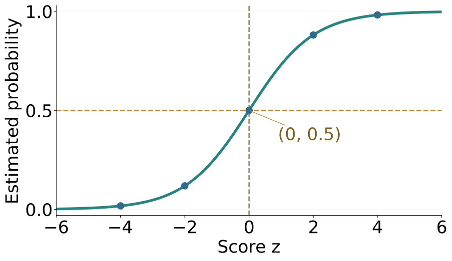
The probability changes smoothly; the class boundary stays linear

\[ \widehat\eta(\boldsymbol{x})\ge\tfrac12 \quad\Longleftrightarrow\quad \boldsymbol{w}^{\mathsf T}\boldsymbol{x}+b\ge0. \]

• A larger positive score means a larger estimated probability of label 1.
• Multiplying all coefficients by 10 keeps the decisions but makes probabilities more extreme.
• An S-shaped probability function does not make this decision boundary curved.

Two minutes. Connect to the sigmoid and its one-half threshold. Confidence and classification are different outputs. For a fixed threshold other than one-half, the boundary is still a hyperplane with a different offset. Do not introduce threshold tuning as another activity here.

The probability model is fixed; now choose the fitting objective

Model: a linear score followed by a sigmoid.

Now: what loss should tell us whether its probabilities fit the labels?

Next: solve for the coefficients that minimize that loss.

30 seconds. Return to the model → objective → solution roadmap. The previous slides defined the output and decision boundary. Accuracy’s flat regions now motivate a smooth probability-fitting objective; log loss is a modeling choice, not an automatic consequence of the sigmoid.

Accuracy gives little guidance between boundary crossings

For one positive review, compare scores \(z=-3\) and \(z=-0.1\).

Score	Predicted probability	Predicted class	Classification error
\(-3\)	4.7%	0	1
\(-0.1\)	47.5%	0	1

The probability moved toward the observed label, but accuracy sees no improvement yet.

A smooth loss can provide information about such changes before the class flips.

Three minutes. Accuracy remains an evaluation criterion. Its stepwise training objective is locally flat almost everywhere, so ordinary gradient updates receive no useful local signal. We are choosing a useful surrogate, not claiming accuracy is an invalid goal or that its optimization is impossible by every method.

Log loss rewards probability assigned to the observed outcome

Let \(a=\widehat\eta(\boldsymbol{x})\) and \(y\in\{0,1\}\).

\[ \ell(y,a)=-y\log a-(1-y)\log(1-a) =\begin{cases}-\log a,&y=1,\\-\log(1-a),&y=0.\end{cases} \]

Give the observed outcome high probability → small loss.

Give the observed outcome nearly zero probability → large loss.

Three minutes. Natural logarithms; a is strictly between zero and one for finite logistic scores. This is binary cross-entropy or negative log likelihood for one Bernoulli observation. Introduce the meaning before deriving the full objective.

Confident mistakes receive a larger penalty

For a positive outcome, \(y=1\):

Predicted probability \(a\)	Class at threshold 0.5	Log loss \(-\log a\)
0.99	Correct	0.010
0.60	Correct	0.511
0.40	Wrong	0.916
0.01	Wrong	4.605

Unlike classification error, log loss distinguishes how confidently a prediction was made.

Two minutes. Have students compare the two wrong predictions and the two correct ones. A single confidently wrong observation can matter greatly; the objective is not simply a count of wrong classifications.

Would accuracy and log loss choose the same model?

Two observed outcomes are both positive: \(y_1=y_2=1\).

Model	Predicted probabilities	Accuracy	Average log loss
A	\((0.60,\;0.60)\)	100%	0.511
B	\((0.99,\;0.49)\)	50%	0.362

What does this comparison establish?

A. Accuracy and log loss always rank models identically.

B. Better log loss can coexist with worse thresholded accuracy.

C. Model B must generalize better to every new population.

B. The criteria assess different outputs. Neither two-example score establishes population performance.

Two minutes. Let students choose, then explain that smooth probability fitting is a surrogate, not an identical numerical version of classification accuracy. Values use natural logs and threshold one-half. Keep the setup short; no calculator task is required because the losses are supplied.

MSE and log loss express different prediction criteria

Numerical regression	Logistic probability prediction
Output: \(\widehat y=z\)	Output: \(a=\sigma(z)\)
Loss: \(\tfrac12(z-y)^2\)	Loss: \(-y\log a-(1-y)\log(1-a)\)
Penalize numerical residual size.	Penalize low probability of the observed label.

Squared error on probabilities is also possible, but composing it with a sigmoid generally loses convexity in the coefficients.

Do not claim squared error is invalid for classification. Brier loss is convex in probability but not generally in logistic coefficients. Convexity will be defined next; here it motivates the question.

The logistic objective has no general closed-form coefficient solution

With \(z_i=\boldsymbol{w}^{\mathsf T}\boldsymbol{x}_i+b\) and \(a_i=\sigma(z_i)=e^{z_i}/(1+e^{z_i})\):

\[\log a_i=z_i-\log(1+e^{z_i}),\qquad \log(1-a_i)=-\log(1+e^{z_i}).\]

\(\displaystyle \ell(y_i,a_i)\)

\(=\)

\(\displaystyle -y_i\log a_i-(1-y_i)\log(1-a_i)\)

(Usual binary log loss)

\(\displaystyle \,\)

\(=\)

\(\displaystyle -y_i z_i+\big[y_i+(1-y_i)\big]\log(1+e^{z_i})\)

(Substitute the two log identities)

\(\displaystyle \,\)

\(=\)

\(\displaystyle \log(1+e^{z_i})-y_i z_i\)

(Combine the coefficients)

Average the same loss over observations:

\[J(\boldsymbol{w},b)=\frac1n\sum_{i=1}^n\ell(y_i,a_i) =\frac1n\sum_{i=1}^n\left[\log(1+e^{z_i})-y_i z_i\right].\]

OLS gave linear stationary equations; logistic loss gives nonlinear equations in the coefficients.

Next: what does the objective’s shape guarantee?

About three minutes before calibration. Start from the ordinary probability-based binary log loss, not an unexplained score formula. Rewrite sigmoid(z)=exp(z)/(1+exp(z)); its complement is 1/(1+exp(z)). Taking logs gives the two displayed identities. Substitution produces -y z + y log(1+exp(z)) + (1-y) log(1+exp(z)); the logarithm coefficients sum to one. Then average over n observations. This is an exact algebraic re-expression, not a new loss or approximation. Natural logs. Finite z gives 0<a<1. There is no general analytic coefficient formula analogous to OLS, though special cases exist. Next is convexity, not immediately gradient descent.

Why the shape of the objective matters

From a solved fit to a fitting algorithm

Stage	Question
1. Interpret the OLS solution	What does the exact fit establish?
2. Choose a classification model and loss	How should a score predict and fit labels?
3. Understand the objective’s shape	When is a local optimum globally best?
4. Compute the coefficients	How can local information guide updates?

30 seconds. Stage 3 of the same four-stage roadmap. Name what the preceding stage established and the question this stage resolves. This guide is orientation, not a new derivation.

Which loss would be easiest to optimize?

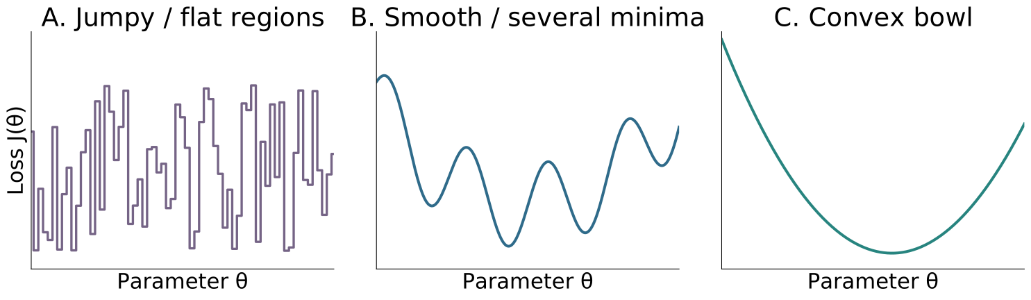
Which shape gives us the clearest route to a global minimum?

A. The jumpy loss.

B. The smooth loss with several minima.

C. The convex bowl.

C. A local minimum is already global; there are no worse local minima to escape.

Two minutes, including the reveal. These are invented one-parameter objectives, not measured model losses. A is a seeded step function: derivatives are zero on flat intervals and undefined at jumps, so a local gradient is not useful. B is a quadratic plus sinusoid with several local minima: smoothness alone does not rule out worse local minima. C is a quadratic. The picture motivates a structural guarantee; it is not a universal runtime comparison.

A useful objective lets us reason about the solution

• Jumpy: a small change may reveal little—or abruptly change the loss.
• Smooth, several minima: downhill progress can end at a worse local minimum.
• Convex: a local minimum is global, making optimality easier to analyze.

Convexity is a useful class of well-behaved objectives.

It gives a global guarantee; speed still depends on the problem and algorithm.

About one minute. An arbitrary objective can hide a better value far from the current point. Without additional structure, local information cannot certify global optimality. Convexity supplies that structure. Do not equate smoothness with convexity or promise that every convex problem is easy to compute. Convex functions can be nonsmooth and can fail to attain a minimum. source:boyd-vandenberghe-convex-optimization.

Objective shape answers three linked questions

1. Define: what does convexity mean geometrically?
2. Check: are our OLS and logistic objectives convex?
3. Interpret: what does that guarantee—and what else do we need?

30 seconds. Connect the next two proofs: the secant inequality defines convexity, and the curvature test gives a practical way to verify it. Then apply the test to our objectives and separate global optimality from uniqueness, existence, and speed.

Convexity is a statement about the entire objective shape

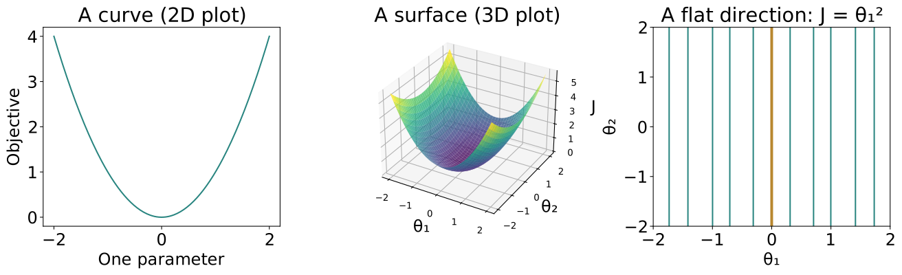
A convex objective may have a single bottom—or a flat set of equally good solutions.

source:boyd-vandenberghe-convex-optimization. Geometric views of the same definition: Left: one parameter, 2D plot. Center: two parameters and height,3D plot. Right: contour view of a flat direction. These are mathematical illustrations, not empirical loss fits.

Definition: a convex function lies below every chord

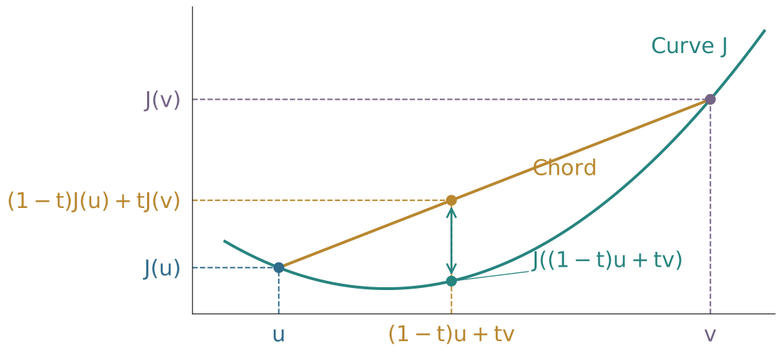
\(J\) is convex on a convex domain if, for every \(\boldsymbol{u},\boldsymbol{v}\) in the domain and \(0\le t\le1\),

\[{\color{#27847f}{J\big(}}{\color{#b8872f}{(1-t)}}{\color{#2f6b8a}{\boldsymbol{u}}}+{\color{#b8872f}{t}}{\color{#756486}{\boldsymbol{v}}}{\color{#27847f}{\big)}} \le {\color{#b8872f}{(1-t)}}{\color{#2f6b8a}{J(\boldsymbol{u})}}+{\color{#b8872f}{t}}{\color{#756486}{J(\boldsymbol{v})}}.\]

Loss at the averaged input ≤ average of the endpoint losses.

source:boyd-vandenberghe-convex-optimization,section3.1.1. Definition, not a claim derived from one drawing. A convex domain contains every weighted average (1-t)u+tv of its points. Plot is the scalar case; bold vectors in the inequality allow multiple coefficients. Blue matches u and J(u), purple matches v and J(v), gold matches both convex combinations. At the same averaged input, the teal curve point is below the gold chord point. The two averages have the same weights but are generally different output values. Point to each labeled axis value before reading the inequality.