Convexity and Numerical Optimization through Adam

ECE 57000 — October 5, 2026

David I. Inouye

Friday connected model, loss, and objective shape

• OLS gives an optimal training fit; redundant features can make coefficients nonunique.
• Logistic regression maps a linear score to a probability and fits it with log loss.
• Convexity means the loss at an averaged input lies below the average endpoint loss.

Today: use that definition to understand optimality, then compute useful updates.

October 2 ended on the chord definition, core/PDF 31. The next proof was briefly previewed and explicitly deferred. Repeat the definition for continuity, then teach the undelivered proof, curvature criterion, Hessian tests, and consequences. About one minute for recap. The two remaining Arc 4 meetings give roughly 100 minutes for about 55–65 minutes of remaining material. Aim through the convergence discussion; a separate regularization/generalization topic and representation limits form the runway. Compare KNN smoothing with coefficient penalties only after optimization and convergence. Keep this next preview private until separately authorized.

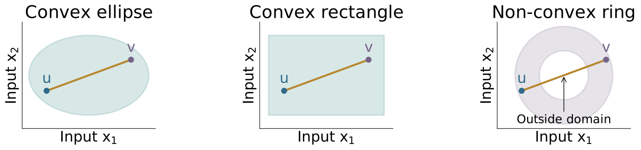
A convex domain contains every segment between its points

A set \(\mathcal D\subseteq\mathbb R^d\) is convex if \[\forall\boldsymbol u,\boldsymbol v\in\mathcal D,\quad\forall t\in[0,1],\quad (1-t)\boldsymbol u+t\boldsymbol v\in\mathcal D.\]

Visual segment test: the entire segment must stay inside the domain for every pair.

source:boyd-vandenberghe-convex-optimization,section2.1. These pictures show allowed input coordinates, not function heights. Filled ellipse and rectangle are convex; the annulus fails because a segment crosses its hole. One failed segment disproves convexity; a few successful segments do not prove it. This input-space requirement makes all the function values in the next chord inequality well-defined. About one minute.

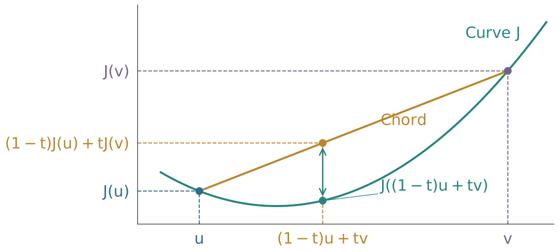
Definition: a convex function lies below every chord

\(J\) is convex on a convex domain if, for every \(\boldsymbol{u},\boldsymbol{v}\) in the domain and \(0\le t\le1\),

\[{\color{#27847f}{J\big(}}{\color{#b8872f}{(1-t)}}{\color{#2f6b8a}{\boldsymbol{u}}}+{\color{#b8872f}{t}}{\color{#756486}{\boldsymbol{v}}}{\color{#27847f}{\big)}} \le {\color{#b8872f}{(1-t)}}{\color{#2f6b8a}{J(\boldsymbol{u})}}+{\color{#b8872f}{t}}{\color{#756486}{J(\boldsymbol{v})}}.\]

Loss at the averaged input ≤ average of the endpoint losses.

source:boyd-vandenberghe-convex-optimization,section3.1.1. Definition, not a claim derived from one drawing. A convex domain contains every weighted average (1-t)u+tv of its points. Plot is the scalar case; bold vectors in the inequality allow multiple coefficients. Blue matches u and J(u), purple matches v and J(v), gold matches both convex combinations. At the same averaged input, the teal curve point is below the gold chord point. The two averages have the same weights but are generally different output values. Point to each labeled axis value before reading the inequality.

Convexity makes every local minimum global

Proof by contradiction. Let \(J\) be convex on a convex domain \(\mathcal D\).

Local minimality at \(\boldsymbol u\) means: for some \(r>0\), \[J(\boldsymbol x)\ge J(\boldsymbol u)\quad\text{whenever }\boldsymbol x\in\mathcal D,\ \|\boldsymbol x-\boldsymbol u\|<r.\]

Suppose \(\boldsymbol u\) is not global: some \(\boldsymbol v\in\mathcal D\) has \(J(\boldsymbol v)<J(\boldsymbol u)\).

Choose \(0<t<\min\{1,r/\|\boldsymbol v-\boldsymbol u\|\}\) and set \(\boldsymbol x_t=(1-t)\boldsymbol u+t\boldsymbol v\).

The segment stays in \(\mathcal D\), and \(\|\boldsymbol x_t-\boldsymbol u\|=t\|\boldsymbol v-\boldsymbol u\|<r\).

\[J(\boldsymbol x_t)\le(1-t)J(\boldsymbol u)+tJ(\boldsymbol v)\quad\text{(convexity)}\]

\[\phantom{J(\boldsymbol x_t)}< (1-t)J(\boldsymbol u)+tJ(\boldsymbol u)=J(\boldsymbol u)\quad\text{(strictly lower loss, }t>0\text{)}.\]

Contradiction: a lower value lies inside the local-minimum neighborhood. Thus \(\boldsymbol u\) is global.

source:boyd-vandenberghe-convex-optimization,section4.2.2. Local minimum is relative to the domain, so boundary points are included. The better value implies v differs from u and the norm denominator is positive. Any t in (0,1) gives strict improvement, but only sufficiently small t guarantees the neighborhood condition. The displayed interval is nonempty. Convexity of the domain keeps the segment feasible. Strictness comes from J(v)<J(u) and t>0, not strict convexity or a strict local minimum. No differentiability, open domain, or uniqueness is required. About three minutes.

For a twice differentiable function, convexity means nonnegative curvature

Let \(J\) be twice continuously differentiable on an open convex domain.

Parameters	Equivalent criterion for convexity
One scalar \(\theta\)	\(J''(\theta)\ge0\) everywhere
A vector \(\boldsymbol{\theta}\)	\(H(\boldsymbol{\theta})=\nabla^2J(\boldsymbol{\theta})\succeq0\) everywhere

The Hessian is the matrix of second partial derivatives: \(H_{jk}=\frac{\partial^2J}{\partial\theta_j\partial\theta_k}\).

Positive semidefinite (PSD) means \(\boldsymbol{v}^{\mathsf T}H\boldsymbol{v}\ge0\) for every direction \(\boldsymbol{v}\). Equivalently, all eigenvalues of \(H\) are \(\ge0\): no eigenvector direction curves downward; zero allows a flat direction at that point.

source:boyd-vandenberghe-convex-optimization,section3.1.4. State the equivalence without deriving it. C2 makes the Hessian symmetric, so its eigenvalues are real. PSD means no direction has negative second-order curvature. Require the criterion everywhere, not only at one candidate minimum. A zero eigenvalue indicates zero second-order curvature at that point, not necessarily a globally flat direction.

Local quadratic approximations reveal the sign of curvature

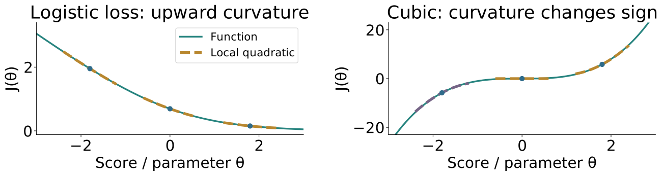
Near any point \(\theta_0\), with \(h=\theta-\theta_0\), \[J(\theta_0+h)=\underbrace{J(\theta_0)+J'(\theta_0)h+\tfrac12J''(\theta_0)h^2}_{\text{local quadratic approximation}}+o(h^2).\]

• Logistic loss: \(J''(\theta)=\sigma(\theta)(1-\sigma(\theta))>0\) at every finite score.
• Cubic: \(J''(\theta)=6\theta<0\) when \(\theta<0\); therefore it is not convex on \(\mathbb R\).

source:boyd-vandenberghe-convex-optimization,section3.1.4. Left: one positive-label logistic loss log(1+exp(-theta)). Right: theta cubed. Solid curves are the functions; short dashed segments are second-order Taylor polynomials at the marked points. They agree in value, slope, and curvature locally, not globally. The formula applies at every point for C2 functions; little-o remainder divided by h squared tends to zero. Upward bending does not mean positive slope or positive function value. The cubic bends downward on the negative half-line and upward on the positive half-line; its zero curvature at zero alone cannot certify convexity. About two minutes.

OLS and logistic log loss have nonnegative directional curvature

Append the intercept to \(\widetilde X\) and the coefficients to \(\boldsymbol{\theta}\).

Objective	Hessian \(H=\nabla^2J\)
OLS	\(\frac1n\widetilde X^{\mathsf T}\widetilde X\)
Logistic log loss	\(\frac1n\widetilde X^{\mathsf T}W\widetilde X\), with \(W_{ii}=a_i(1-a_i)\ge0\)

For logistic loss, \(\ell(z,y)=\log(1+e^z)-yz\) gives \(\ell'=\sigma(z)-y\) and \(\ell''=a(1-a)\).

\[\boldsymbol{v}^{\mathsf T}H\boldsymbol{v} =\frac1n\sum_i a_i(1-a_i)(\widetilde{\boldsymbol{x}}_i^{\mathsf T}\boldsymbol{v})^2\ge0.\]

For OLS, replace the weights by 1. Both objectives are convex in the coefficients.

source:boyd-vandenberghe-convex-optimization. The intercept-augmented observation is a column vector; its transpose is a row of Xtilde. Derive scalar logistic derivatives directly from log(1+exp(z)); sigmoid prime=a(1-a). Outer-product chain rule yields Hessian. Adding lambda/2||w||² adds a PSD diagonal block, preserving convexity.

Convexity makes a local optimum globally meaningful

• Local minimum → global minimum. Zero gradient also certifies a global minimum for a differentiable convex objective.
• Uniqueness needs more: strict convexity excludes multiple minimizers, if a minimizer exists.
• Existence needs more: a convex loss can approach its infimum without attaining it.

Next: a useful shape does not itself tell us how to compute the solution.

source:boyd-vandenberghe-convex-optimization,chapters3,4,9. First-order tangent bound J(v)>=J(u)+gradJ(u)^T(v-u); zero gradient lower-bounds every other value by J(u). Derive tangent bound by taking t->0 in secant inequality if asked. Do not cover smoothness constants or convergence-rate guarantees. Existence and uniqueness are distinct from global optimality.

Fitting models with local information

A well-behaved shape still requires a numerical route to the solution

OLS: solve linear normal equations.

Logistic regression: repeatedly evaluate and improve the coefficients.

The objective is convex; our next task is to turn local information into useful steps.

30 seconds. Arc4 stage4. Numerical methods are not limited to GD, but it is the central reusable method for later models.

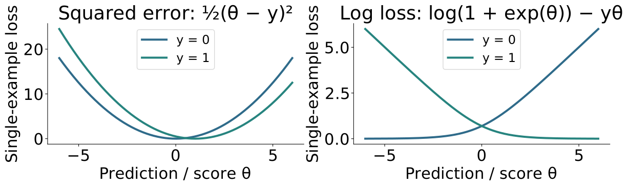
Logistic loss has flatter tails than squared error

• Each curve is the loss for one example, with its label fixed at \(y=0\) or \(y=1\).
• Squared error has constant curvature; log loss flattens toward a confident correct prediction.
• For \(y=1\), log loss decreases as the score grows; for \(y=0\), it decreases as the score falls.

Analytic per-example curves, not an average over conflicting labels. For squared error theta is the numerical prediction; for logistic loss theta is the pre-sigmoid score. Vertical scales differ. A dataset objective averages its examples’ loss curves; its shape depends on their inputs and labels. Separable data need not give a finite minimizer. No coefficient penalty is used.

A derivative predicts the effect of a small parameter change

First-order Taylor expansion centered at \(\theta\), for a small change \(\Delta\):

\[J(\theta+\Delta)\approx J(\theta)+J'(\theta)\Delta.\]

• If \(J'(\theta)>0\), a small negative change reduces the objective.
• If \(J'(\theta)<0\), a small positive change reduces it.
• This is a local approximation, not a prediction for an arbitrary step.

Three minutes. Bridge familiar scalar derivatives to their computational role. Theta is an illustrative scalar parameter, not a random variable. Draw a tangent line and explain what “small” means geometrically. The learning-rate issue follows.

A gradient collects the partial derivatives

Bundle the parameters into \(\boldsymbol{\theta}=(w_1,\ldots,w_d,b)^{\mathsf T}\).

\[ \nabla J(\boldsymbol{\theta})= \begin{bmatrix} \partial J/\partial w_1 & \cdots & \partial J/\partial w_d & \partial J/\partial b \end{bmatrix}^{\mathsf T}. \]

For a small vector change \(\boldsymbol{\Delta}\):

\[J(\boldsymbol{\theta}+\boldsymbol{\Delta}) \approx J(\boldsymbol{\theta})+\nabla J(\boldsymbol{\theta})^{\mathsf T}\boldsymbol{\Delta}.\]

The gradient has one component per parameter.

Three minutes. Each partial derivative changes one parameter while fixing the others. Connect shapes to Arc 2: the inner product produces one scalar predicted change in the objective. Different feature scales change gradient magnitudes.

Moving against the gradient gives local descent

For \(\alpha>0\), choose \(\boldsymbol{\Delta}=-\alpha\nabla J(\boldsymbol{\theta})\).

\[ \nabla J(\boldsymbol{\theta})^{\mathsf T}\boldsymbol{\Delta} =-\alpha\|\nabla J(\boldsymbol{\theta})\|_2^2\le0. \]

This motivates the repeated update

\[\boldsymbol{\theta}_{t+1}=\boldsymbol{\theta}_t-\alpha\nabla J(\boldsymbol{\theta}_t).\]

Next: inspect what these finite steps do when we can see only the local slope.

Three minutes. Strictly negative when the gradient is nonzero. The inequality concerns the first-order predicted change; a finite step can still increase the actual objective. For the convex objectives just established, a zero gradient establishes global optimality; a finite step still needs an appropriate learning rate. Do not skip the derivative of sigmoid/log loss when deriving the logistic update next class. Numerical convergence and generalization remain separate.

Small steps follow the local downhill direction

Same objective, same starting point. Learning rate: \(\alpha=2.0\).

The algorithm sees this point and this slope.

A negative-gradient step uses that local information.

Gold segments show only the slopes we have evaluated.

The objective falls; the slope keeps its sign.

Three steps approach the minimum.

Two minutes. Initial state: one point and tangent, no curve. Click 1 animates the first update and reveals the answer; click 2 reveals the next update; click 3 the final landing; click 4 reveals the entire curve. Exactly three tangent segments are accumulated, at theta_0, theta_1, theta_2, with a final landing point theta_3. The dashed connectors show jumps, not an evaluated path or the objective curve. Axes are scaled separately for readability; do not compare visual steepness across slides.

The same unregularized logistic objective is used throughout: J(theta)=log(1+exp(theta))-theta/2. Two observations have x=1, labels 0 and 1, score theta, no separate intercept. Its derivative is sigmoid(theta)-1/2. The stationary minimum is theta=0; curvature is at most 1/4 and tends to zero in the tails. Alpha=2 gives a monotone approach; alpha=6 gives shrinking alternating steps; alpha=12 increases loss on the first step, then keeps oscillating and a bounded nonzero two-cycle in the long run. This is failure to converge, not unbounded divergence. No penalty is needed. A finite-data logistic objective has bounded gradients; do not describe the first few rising losses as a proof of unbounded divergence.

Step	theta	objective	slope
0	2.000	1.127	+0.381
1	1.238	0.874	+0.275
2	0.688	0.751	+0.165
3	0.357	0.709	+0.088

\(\theta_{t+1}=\theta_t-\alpha J'(\theta_t)\) · Unregularized logistic loss · Three updates; the first three evaluated slopes remain visible.

What happens after this larger step?

Same objective, same starting point. Learning rate: \(\alpha=6.0\).

After the next update, what happens?

A. Objective decreases; slope keeps its sign.
B. Objective decreases; slope reverses sign.
C. Objective increases; slope keeps its sign.
D. Objective increases; slope reverses sign.

B. The objective falls, but the slope reverses: we jumped across the valley.

Three steps approach the minimum.

Three minutes including the four-choice question; instructor explicitly overrides the three-choice guidance. Initial state: one point and tangent, no curve. Click 1 animates the first update and reveals the answer; click 2 reveals the next update; click 3 the final landing; click 4 reveals the entire curve. Exactly three tangent segments are accumulated, at theta_0, theta_1, theta_2, with a final landing point theta_3. The dashed connectors show jumps, not an evaluated path or the objective curve. Axes are scaled separately for readability; do not compare visual steepness across slides.

The same unregularized logistic objective is used throughout: J(theta)=log(1+exp(theta))-theta/2. Two observations have x=1, labels 0 and 1, score theta, no separate intercept. Its derivative is sigmoid(theta)-1/2. The stationary minimum is theta=0; curvature is at most 1/4 and tends to zero in the tails. Alpha=2 gives a monotone approach; alpha=6 gives shrinking alternating steps; alpha=12 increases loss on the first step, then keeps oscillating and a bounded nonzero two-cycle in the long run. This is failure to converge, not unbounded divergence. No penalty is needed. A finite-data logistic objective has bounded gradients; do not describe the first few rising losses as a proof of unbounded divergence.

Step	theta	objective	slope
0	2.000	1.127	+0.381
1	-0.285	0.703	-0.071
2	0.140	0.696	+0.035
3	-0.069	0.694	-0.017

\(\theta_{t+1}=\theta_t-\alpha J'(\theta_t)\) · Unregularized logistic loss · Three updates; the first three evaluated slopes remain visible.

What happens when we take an even larger step?

Same objective, same starting point. Learning rate: \(\alpha=12.0\).

After the next update, what happens?

A. Objective decreases; slope keeps its sign.
B. Objective decreases; slope reverses sign.
C. Objective increases; slope keeps its sign.
D. Objective increases; slope reverses sign.

D. The objective rises and the slope reverses: we jumped too far.

Continuing these updates settles into an oscillation instead of reaching the minimum.

Three minutes including the four-choice question; instructor explicitly overrides the three-choice guidance. Initial state: one point and tangent, no curve. Click 1 animates the first update and reveals the answer; click 2 reveals the next update; click 3 the final landing; click 4 reveals the entire curve. Exactly three tangent segments are accumulated, at theta_0, theta_1, theta_2, with a final landing point theta_3. The dashed connectors show jumps, not an evaluated path or the objective curve. Axes are scaled separately for readability; do not compare visual steepness across slides.

The same unregularized logistic objective is used throughout: J(theta)=log(1+exp(theta))-theta/2. Two observations have x=1, labels 0 and 1, score theta, no separate intercept. Its derivative is sigmoid(theta)-1/2. The stationary minimum is theta=0; curvature is at most 1/4 and tends to zero in the tails. Alpha=2 gives a monotone approach; alpha=6 gives shrinking alternating steps; alpha=12 increases loss on the first step, then keeps oscillating and a bounded nonzero two-cycle in the long run. This is failure to converge, not unbounded divergence. No penalty is needed. A finite-data logistic objective has bounded gradients; do not describe the first few rising losses as a proof of unbounded divergence.

Step	theta	objective	slope
0	2.000	1.127	+0.381
1	-2.570	1.359	-0.429
2	2.577	1.362	+0.429
3	-2.575	1.361	-0.429

\(\theta_{t+1}=\theta_t-\alpha J'(\theta_t)\) · Unregularized logistic loss · Three updates; the first three evaluated slopes remain visible.

The gradient is an average of example contributions

If \(J(\boldsymbol{\theta})=\frac1n\sum_i\ell_i(\boldsymbol{\theta})\), then

\[\nabla J(\boldsymbol{\theta})=\frac1n\sum_i\nabla\ell_i(\boldsymbol{\theta}).\]

Update	Examples used for one gradient estimate
Full-batch GD	All \(n\) examples
Single-example SGD	One randomly sampled example
Mini-batch SGD	A small randomly sampled group \(B\)

All use \(\boldsymbol{\theta}_{t+1}=\boldsymbol{\theta}_t-\alpha_t\boldsymbol{g}_t\).

Minibatch is the intended third category; batchGD conventionally means fullbatch. With a fixed regularizer, add its gradient once to each estimate, not once per sampled loss without normalization.

Sampling trades exact direction for cheaper, noisy updates

For uniform sampling at the current parameters:

\[\boldsymbol{g}_B=\frac1{|B|}\sum_{i\in B}\nabla\ell_i(\boldsymbol{\theta}), \qquad \mathbb E_B[\boldsymbol{g}_B\mid\boldsymbol{\theta}]=\nabla J(\boldsymbol{\theta}).\]

• One stochastic step can increase the full training objective.
• Larger batches usually reduce gradient noise but cost more per update.
• Compare runs by examples processed or time, not only update count.

A fixed learning rate can leave persistent fluctuations near the minimum.

Uniform independent draws or a uniformly chosen subset give the unbiased mean at fixed theta. Sequential random reshuffling has a more nuanced conditional statement. Declining step sizes can improve settling under appropriate conditions.

Adam averages directions and adapts each coordinate scale

For the current gradient estimate \(\boldsymbol{g}_t\):

\[\boldsymbol{m}_t=\beta_1\boldsymbol{m}_{t-1}+(1-\beta_1)\boldsymbol{g}_t, \qquad \boldsymbol{v}_t=\beta_2\boldsymbol{v}_{t-1}+(1-\beta_2)\boldsymbol{g}_t^2.\]

The hats correct the initial bias from \(\boldsymbol m_0=\boldsymbol v_0=\boldsymbol 0\): \[\widehat{\boldsymbol m}_t=\frac{\boldsymbol m_t}{1-\beta_1^t},\qquad \widehat{\boldsymbol v}_t=\frac{\boldsymbol v_t}{1-\beta_2^t}.\]

\[\boldsymbol{\theta}_{t+1}=\boldsymbol{\theta}_t- \alpha\frac{\widehat{\boldsymbol{m}}_t}{\sqrt{\widehat{\boldsymbol{v}}_t}+\epsilon}.\]

Average the recent directions; rescale coordinates with large recent squared gradients.

The base learning rate still matters. Adaptation is not a convergence guarantee.

source:kingma-ba-adam. Elementwise square/root/division. Initialize m0=v0=0; hats correct initial bias: mhat=mt/(1-beta1^{t),vhat=vt/(1-beta2}t). beta values weight history; epsilon prevents division by zero. Do not teach an optimizer catalog or transfer vanilla convex-GD guarantees to Adam. AdamW is a later optional note on decoupled weight decay.