Fitting Models with Local Information (continued)

ECE 57000 — October 9, 2026

David I. Inouye

Monday connected objective shape and practical updates

• Convexity makes every local minimum global; existence and uniqueness need more.
• Gradients give local information: step size controls whether an update helps.
• Mini-batches trade computation for noise; Adam averages and rescales gradients.

Today: fit logistic regression, diagnose convergence, and separate optimization from generalization.

October 5 ended on Adam (PDF slide 21); the logistic-gradient slide was previewed and deferred until after the exam. Allow about a minute each for recap and Adam. Finish Arc 4’s logistic gradients, convergence, regularization, and model-limits audit (roughly 30–40 minutes at recent pace). Then teach the nonlinear-representation opening through the two-ReLU construction: expected stop at PDF slide 27, roughly 50–60 minutes total after adding the real-image motivation. Thirteen authored runway slides continue with matrix form, dimensions, readouts including softmax, composition, affine collapse, measured product-image evidence, and credit assignment (about 25–30 minutes). Keep the two live checks; optional algebra can stay in notes. The automated timing heuristic is shorter than recent delivery: use the room’s pace rather than hurrying to the marker. Keep this deck private until separately authorized for preview deployment.

Adam averages directions and adapts the step size for each parameter

For the current gradient estimate \(\boldsymbol{g}_t\):

\[\boldsymbol{m}_t=\beta_1\boldsymbol{m}_{t-1}+(1-\beta_1)\boldsymbol{g}_t, \qquad \boldsymbol{v}_t=\beta_2\boldsymbol{v}_{t-1}+(1-\beta_2)\boldsymbol{g}_t^2.\]

The hats correct the initial bias from \(\boldsymbol m_0=\boldsymbol v_0=\boldsymbol 0\): \[\widehat{\boldsymbol m}_t=\frac{\boldsymbol m_t}{1-\beta_1^t},\qquad \widehat{\boldsymbol v}_t=\frac{\boldsymbol v_t}{1-\beta_2^t}.\]

\[\boldsymbol{\theta}_{t+1}=\boldsymbol{\theta}_t- \alpha\frac{\widehat{\boldsymbol{m}}_t}{\sqrt{\widehat{\boldsymbol{v}}_t}+\epsilon}.\]

Average the recent directions; reduce the step size for parameters with large recent squared gradients.

The base learning rate still matters. Adaptation is not a convergence guarantee.

source:kingma-ba-adam. Elementwise square/root/division. Initialize m0=v0=0; hats correct initial bias: mhat=mt/(1-beta1^{t),vhat=vt/(1-beta2}t). beta values weight history; epsilon prevents division by zero. Do not teach an optimizer catalog or transfer vanilla convex-GD guarantees to Adam. AdamW is a later optional note on decoupled weight decay.

The logistic objective has a directly computable gradient

Include the intercept in \(\widetilde{\boldsymbol x}_i=(\boldsymbol x_i^{\mathsf T},1)^{\mathsf T}\) and \(\boldsymbol\theta=(\boldsymbol w^{\mathsf T},b)^{\mathsf T}\); let \(a_i=\sigma(\boldsymbol\theta^{\mathsf T}\widetilde{\boldsymbol x}_i)\).

\[J(\boldsymbol\theta)=-\frac1n\sum_{i=1}^n\big[y_i\log a_i+(1-y_i)\log(1-a_i)\big],\qquad \nabla_{\boldsymbol\theta}J=\frac1n\sum_{i=1}^n(a_i-y_i)\widetilde{\boldsymbol x}_i.\]

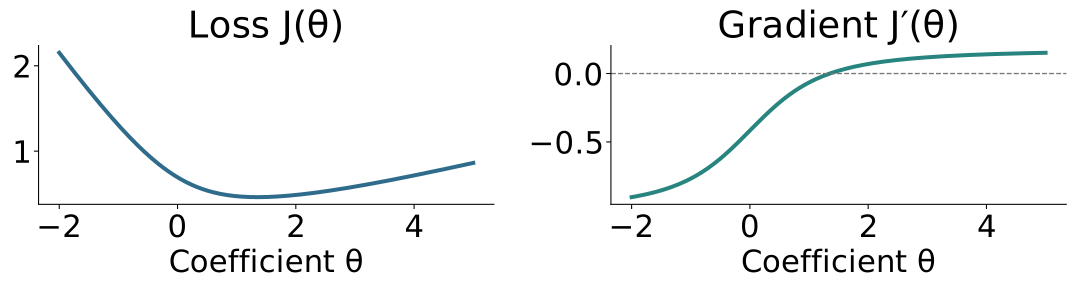
One-coefficient example: \(a_i=\sigma(\theta x_i)\), no intercept; \(J'(\theta)=\frac1n\sum_i(\sigma(\theta x_i)-y_i)x_i\).

Direct result of elementary chain rule and algebra; omit intermediate sigmoid and log derivatives. Vector theta contains d+1 parameters and gradient has the same dimension. The figure uses x=(-2,-1,-.5,.5,1,2), y=(0,0,1,0,1,1), no intercept and no penalty. All inputs are distinct. Solid curves show actual mean log loss and its analytic derivative. The next convergence experiment also fits an intercept. Use the gradient sign and zero crossing to connect the panels.

Each example contributes prediction error times its input

\[\nabla J(\boldsymbol\theta)=\frac1n\sum_i\underbrace{(a_i-y_i)}_{\text{probability residual}}\widetilde{\boldsymbol x}_i, \qquad \boldsymbol\theta_{t+1}=\boldsymbol\theta_t-\alpha\nabla J(\boldsymbol\theta_t).\]

• Underpredict a positive label: \(a_i-y_i<0\); that example’s descent contribution raises its score.
• Overpredict a negative label: \(a_i-y_i>0\); its descent contribution lowers its score.
• Average these contributions: examples can pull in different directions; larger feature values amplify the corresponding gradient entry.

Now watch the full training objective change over repeated updates.

For a single example, the score change from its descent contribution is proportional to -(a-y)||xtilde||^2. In a batch, other examples can counteract it; do not claim every example improves on each full-batch update. The intercept contribution uses the appended input 1. Learning rate controls the size of the combined step. No penalty or intermediate calculus derivation here.

Return to logistic regression and watch the fit evolve

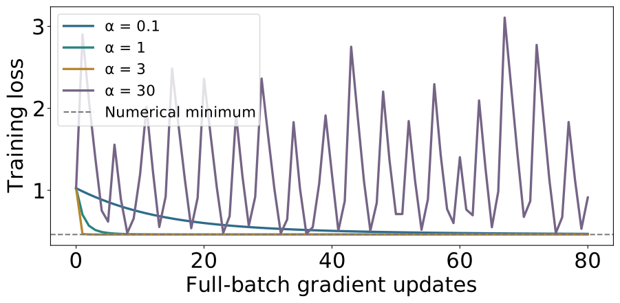
Small illustrative dataset: six inputs \(x=(-2,-1,-0.5,0.5,1,2)\) and labels \(y=(0,0,1,0,1,1)\).

\[a_i=\sigma(wx_i+b),\qquad J(w,b)=\frac16\sum_i\ell(y_i,a_i).\]

Start every run at \((w,b)=(-0.5,0.8)\) and change only the learning rate.

The overlapping labels give a finite minimum without a coefficient penalty.

This six-point dataset is explicitly illustrative, not a subset of review data. Reference solution computed with BFGS to high accuracy; curves are actual full-batch GD runs. No regularization is used.

A linear loss axis shows large early improvements

Small steps are slow; larger useful steps improve quickly; oversized steps can keep oscillating.

Reference is a numerical minimum, not held-out error. The oversized-step trajectory fails to approach the minimum; the plot includes its full range. Same initialization and data for all learning rates.

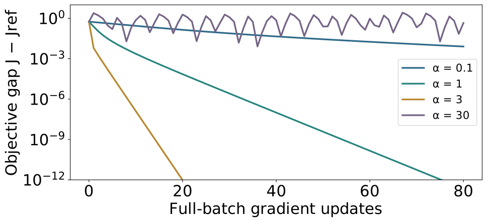
A log gap axis reveals progress near the minimum

Equal vertical distances now represent multiplicative changes in \(J-J_{\mathrm{ref}}\).

Jref is high-accuracy numerical reference, not an analytic answer or true population loss. Positive gaps below1e-14 are floored only for plotting; displayed lower range1e-12 avoids interpreting roundoff as progress. The oversized-step run has a persistent objective gap.

Convergence means little useful optimization remains

Check both a small gradient and small sustained changes in the objective.

• A visually flat trace alone may reflect a tiny learning rate or poor scaling.
• With a finite convex optimum, solving to useful tolerance is a sensible stopping point.
• Optimization progress is measured on training loss; generalization needs held-out evidence.

Near-zero loss does not automatically mean “finished”: separable logistic fits and large deep models need more care.

Do not claim a small gradient universally gives a tight distance-to-optimum bound without curvature assumptions. A strong-convexity bound can make that quantitative, but is beyond this introduction. Keep deep-model preview brief; neither zero loss nor further training guarantees good generalization.

Does a flat loss trace show convergence?

Training loss barely changes over 100 updates, but the gradient norm remains large.

What should you check next?

A. Whether the learning rate is tiny or the features are poorly scaled.

B. Whether a stronger penalty can certify convergence to the same objective.

C. Whether the flat trace alone is enough to stop optimizing.

A. Small updates can hide a substantial remaining descent direction.

Two-minute commitment-and-reveal question. Answer A. The distinction is numerical stagnation versus useful convergence; a small objective change alone is insufficient. B changes the objective and C mistakes appearance for evidence. Ask students to connect the gradient, step size, and actual parameter change. No universal objective-gap bound follows without additional curvature assumptions.

Controlling model complexity for generalization

Better training fit can mean worse prediction on new data

We have learned how to minimize a training objective.

The ML goal is still performance on new examples.

Regularization limits how freely a model can fit the training data, trading some flexibility for potentially better generalization.

Recall KNN: a tiny neighborhood can follow sample-specific fluctuations.

Connect back to Arc 3 rather than introduce regularization as an optimizer trick. Regularization is broader than adding a penalty. It can improve prediction when the restriction suppresses irrelevant variation, but excessive restriction underfits. No universal guarantee of improved test performance.

Larger KNN neighborhoods and coefficient penalties both control flexibility

Mechanism	Weaker restriction	Stronger restriction
KNN neighborhood size \(k\)	Small \(k\): follow nearby examples closely	Large \(k\): average over more examples
Coefficient penalty strength \(\lambda\)	Small \(\lambda\): allow larger coefficients	Large \(\lambda\): discourage large coefficients

For a linear model, one common choice is L2 regularization:

\[J_\lambda(\boldsymbol{w},b)=J_{\mathrm{train}}(\boldsymbol{w},b)+\frac\lambda2\|\boldsymbol{w}\|^2.\]

Different mechanisms, same purpose: control sensitivity to the training sample.

Too much restriction can hide useful signal. \(k\) and \(\lambda\) have no numerical equivalence.

source:boyd-vandenberghe-convex-optimization. Here the intercept is unpenalized and features must be scaled sensibly. KNN is implicit smoothing; L2 is an explicit penalty. Neither changes the underlying objective of ML: useful held-out prediction. The penalty changes the fitted solution, unlike learning rate alpha, which controls the numerical route to a fixed objective. Penalties can also affect conditioning or ensure finite solutions, but these are secondary effects here.

Both mechanisms can improve held-out prediction

Ames KNN using living area only — validation RMSE:

\(k=1\)	\(k=100\)	\(k=1758\) (all training sales)
$75,300	$57,700	$80,200

Ames linear models using 226 encoded features — test RMSE:

No penalty: OLS	L2 penalty: validation-selected ridge
$26,300	$25,600

Compare within each row: these use different representations and evaluation splits.

The restriction can help; the strongest restriction need not be best.

source:ames-housing-data; source:ames-housing-documentation. Existing fixed seed570, 1758/586/586 split. KNN numbers from ames-knn-complexity.json: 75304.58, 57676.68, 80158.28; k=100 was selected from the original candidate grid using validation. This row illustrates tuning, not an unbiased final test estimate. Ridge versus OLS from ames-regression.json: test26279.26 versus25566.97, validation-selected sklearn Ridge alpha10 with train-only preprocessing. Library alpha uses a sum-loss convention and is not numerically the lambda in our mean-loss equation. No across-row ranking or universal superiority claim. The real Cornell classifier also used an L2 penalty; today’s unregularized examples isolated optimization behavior.

Choose the restriction with validation; assess the choice on test data

1. Fit: train each candidate using only training observations.
2. Choose: compare candidates on validation data.
3. Assess: evaluate the selected procedure on untouched test data.

Search positive \(\lambda\) values on a log scale: multiply, rather than add.

Search	Example \(\lambda\) values
Broad search: factors of 10	\(10^{-4},10^{-3},10^{-2},10^{-1},1,10,100\)
Refine near a promising \(\lambda=1\)	\(0.1,0.3,1,3,10\)

Common mistake: \(0,1,2,3,\ldots\) misses the entire range \(0<\lambda<1\).

Include \(\lambda=0\) separately as the no-penalty baseline; zero has no logarithm.

Revisit the existing split protocol briefly. Budget about three minutes, including the tuning example. Positive penalty strengths often need exploration across orders of magnitude: equal ratios cover relative scales that equal increments can miss. The displayed grids are illustrative, not universal bounds. Standardize features using training statistics; the appropriate lambda range depends on feature scaling and the loss/penalty normalization. If the best validation result is at a grid boundary, expand in that direction; otherwise refine around the promising region. The second grid is approximately logarithmically spaced (factors near three) and is an example of refinement, not evidence that lambda=1 is optimal. Check lambda=0 separately when an unregularized fit is well-defined. Choose the entire search using validation data and inspect test performance only after selection.

Learning rate controls how we approach a chosen objective; regularization changes which fitted solution we prefer. Optimization should be sufficiently accurate for a fair comparison; an under-converged candidate can confuse an optimization failure with a poor regularization choice. Validation-guided early stopping can itself act as regularization, but defer its details. Improving test performance is a measured outcome, not something every penalty guarantees.

Better optimization cannot repair the wrong function class

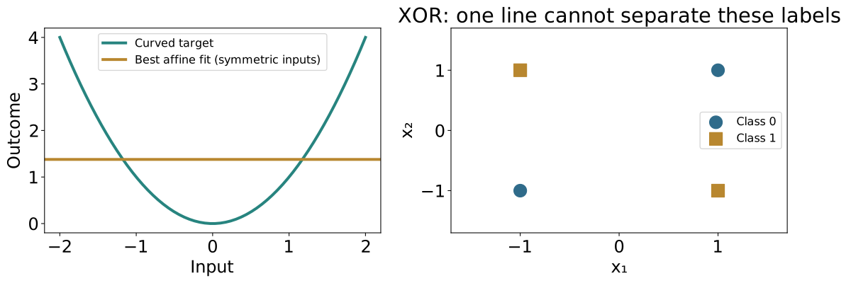
A curved numerical pattern and XOR labels cannot be represented by one affine predictor.

Illustrative analytic examples. Left line is leastsquares for symmetric inputs with squared target. Right contradictory inequalities show no affine classifier separates XOR; optional board proof using average of each class at origin. Distinguish representation failure from an unfinished fit.

The next arc changes the function we can represent

We now have: models → objectives → exact or numerical fitting → evaluation.

The remaining limitation: a single affine map cannot express every useful pattern.

Next task: categorize real product images. Can learned nonlinear features improve the predictor?

We will use XOR to explain the mechanism, then return to the real images.

30-second closing handoff to Arc5. No deep-learning machinery required before this point.

Learning nonlinear representations

A product image must become a useful category

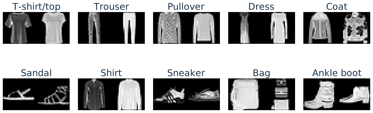
A catalog task: assign a product image to a category such as shirt, bag, or shoe.

Fashion-MNIST: \(28\times28\) grayscale images, 784 pixel features, ten categories.

Zalando Research, Fashion-MNIST

About two minutes. [Sources] source:fashion-mnist; source:fashion-mnist-train-images; source:fashion-mnist-train-labels. These are actual product images, not generated illustrations. The benchmark contains 60,000 official training images and 10,000 test images. The figure uses the first two images of each class in our fixed training subset, without choosing examples using predictions. Ask students to notice variation within a category and resemblance across categories as an informal observation, not an additional live poll. Product catalog classification motivates the task, but this clean, low-resolution, single-item benchmark does not establish production performance on arbitrary seller photos, backgrounds, or unknown categories. Full benchmark classes are retained; do not select an easy or difficult binary pair after looking at results.

Softmax and cross-entropy extend binary logistic regression

For image \(\boldsymbol x\in[0,1]^{784}\) and category \(c=1,\ldots,10\):

1. Compute an affine score: \(s_c=\boldsymbol w_c^{\mathsf T}\boldsymbol x+b_c\).

2. Apply softmax to turn the scores into probabilities that sum to one:

\[p_c=\frac{\exp(s_c)}{\sum_{j=1}^{10}\exp(s_j)}.\]

3. Use cross-entropy: if the true category is \(y\), penalize low \(p_y\):

\[\ell(y,\boldsymbol p)=-\log p_y,\qquad J=\frac1n\sum_{i=1}^n-\log p_{i,y_i}.\]

Softmax generalizes sigmoid; cross-entropy generalizes binary log loss.

About three minutes. Define p_c as the probability assigned to category c for this image, y as its true category index, and p_{i,y_i} as example i’s probability for its true category. Predict the largest probability, equivalently the largest score. Average cross-entropy is the unpenalized data objective; the next slide fits candidates with an L2 weight penalty as in the prior regularization section. No one-hot notation is needed. In the two-class case p_1=sigma(s_1-s_2), so fixing one reference score recovers the earlier sigmoid model. For a one-hot true label, multiclass cross-entropy is exactly -log p_y; the binary expression -y log a-(1-y)log(1-a) selects the same true-label probability. Subtract the maximum score in numerical softmax implementations. Although the probabilities are nonlinear in x, pairwise decision boundaries s_c=s_j remain affine: the linear classifier terminology refers to its scores and boundaries. Do not call a sigmoid or softmax alone a learned nonlinear feature representation. [Sources] source:fashion-mnist; source:d2l-multilayer-perceptrons. Flattening and division by255 retain the image information. The same ten-score probability/loss construction is reused after hidden features later.

Regularization helps, but a nonlinear model improves validation accuracy

Same 12,000 training and 3,000 validation images; same pixel features.

Model	Training accuracy	Validation accuracy
Linear, \(C=0.01\) (stronger penalty)	84.66%	82.37%
Linear, \(C=0.1\)	88.70%	84.03%
Linear, \(C=1\)	92.21%	82.73%
Linear, \(C=10\) (weaker penalty)\(^*\)	94.90%	80.40%
Nonlinear model	94.10%	85.70%

\(C\) is inverse regularization strength. \(^*\)This fit reached its iteration limit.

How do we go beyond linear functions, and why can that help?

A tiny image task will make the missing interaction explicit.

About two minutes. [Sources] source:fashion-mnist; source:fashion-mnist-train-images; source:fashion-mnist-train-labels. These are the actual candidate results in fashion-mnist-results.json, not test accuracies. C is sklearn’s inverse penalty parameter: increasing C weakens regularization. Do not identify C numerically with the earlier lambda. The first three linear fits converged; C10 reached1500 iterations, is explicitly flagged, and was not selected. As the penalty weakens, training accuracy rises while validation need not improve. Among the tried linear settings, C0.1 is selected by validation. The nonlinear row is a one-hidden-layer 64-ReLU MLP with alpha0.01, selected among .0001,.01,1; architecture and 60-epoch Adam budget were fixed beforehand. Defer its internals until after XOR. Its training budget is not a convergence claim. Validation-selected accuracy is used to motivate/model-select, not as an unbiased final estimate; the later comparison uses official test data. No test outcomes were used for these choices. The observed gap motivates investigating learned features; it does not prove that every linear model must be worse, nor that the real dataset is literally XOR. Distinguish nonlinear probabilities from nonlinear scores, as on the preceding slide.

An image label can depend on relationships between regions

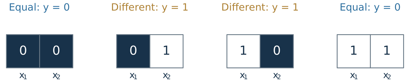
To isolate the mechanism, use a toy image task: flag a mismatch between two regions.

Represent their brightness by \(\boldsymbol{x}=[x_1,x_2]^{\mathsf T}\in\{0,1\}^2\).

Predict \(y=1\) when the regions differ; otherwise predict \(y=0\).

Bridge from the real product-image task to an exact, deliberately tiny example. This is an original two-pixel illustration, not a Fashion-MNIST sample or an empirical claim. Dark means0 and bright means1. Each square can also stand for one measured image region. The exact four cases are the complete task; no train/test performance is claimed. About two minutes. [Sources] source:d2l-multilayer-perceptrons, section5.1.1.1 motivates context-dependent image features; the construction and figures are original.

A raw affine score gives each pixel one fixed contribution

\[z=w_1x_1+w_2x_2+b,\qquad a=\sigma(z).\]

Changing \(x_1\) from 0 to 1 changes the score by \(w_1\), whatever \(x_2\) is.

Other region	What the mismatch task needs when \(x_1:0\to1\)
\(x_2=0\)	Class changes from 0 to 1
\(x_2=1\)	Class changes from 1 to 0

A monotone sigmoid cannot make the same score increment point both ways.

This is a limitation of this model on the defined XOR task, not a claim that all image tasks defeat affine predictors. Use the usual probability threshold1/2, equivalent to score threshold zero. A nonzero fixed w1 raises both scores or lowers both scores; zero changes neither. The sigmoid changes the magnitude of the probability response with context, but not its direction. About two minutes. [Sources] source:d2l-multilayer-perceptrons, section5.1.1.1. Original four-case argument.

XOR cannot be separated by one straight decision line

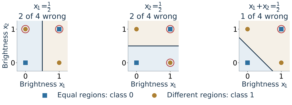
Toy image: two brightness features \(x_1,x_2\in\{0,1\}\). Label different regions 1, equal regions 0.

Shading shows predictions; markers show true classes. Red rings mark errors.

No single straight decision line separates the two classes.

About two minutes. Keep the preceding image setup and fixed-contribution explanation; this slide supplies the geometric intuition. Each panel predicts1 when w1x1+w2x2+b>0: weights [1,0], [0,1], [1,1], with b=-1/2. Blue shading predicts0; gold predicts1. Filled squares/circles show true classes; red rings mark mistakes. Vertical and horizontal lines each miss two examples; the diagonal misses [1,1]. These candidate failures illustrate the limitation, rather than exhaustively testing every line. The previous slide supplies the general argument: changing x1 has the same signed effect on the affine score regardless of x2, whereas XOR requires opposite class changes. Moving or rotating one line cannot fix this. No additional geometric proof is needed here. [Sources] source:d2l-multilayer-perceptrons. Candidate constructions and figure are original.

A difference feature makes the same labels easy to separate

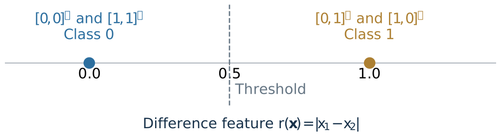
Choose the feature \(r(\boldsymbol{x})=|x_1-x_2|\).

\[\widehat y=\mathbb 1\{r(\boldsymbol{x})>\tfrac12\}.\]

We changed the representation, not the four labels or the fitting algorithm.

About two minutes. Define the indicator as one when its condition is true and zero otherwise. The feature is hand chosen to expose the mechanism; do not imply it was learned. Feature maps can discard information: both equal-brightness images map to zero, which is appropriate for this task but not for every task. Next ask how to express such a feature using reusable trainable parts. [Sources] source:d2l-multilayer-perceptrons, section5.1.1.2 for learned representations; this absolute-difference construction is original.

A neuron applies a nonlinear function to an affine score

\[s=\boldsymbol{w}^{\mathsf T}\boldsymbol{x}+b,\qquad h=\phi(s).\]

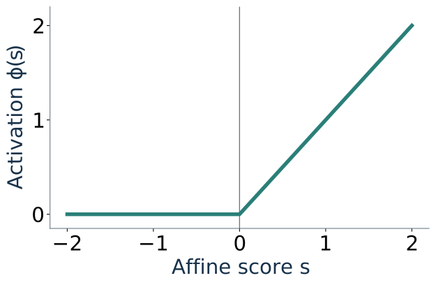
Rectified linear unit (ReLU):

\[\phi(s)=\max(0,s).\]

For \(\boldsymbol{w}=[1,-1]^{\mathsf T}\) and \(b=0\):

\[h=\max(0,x_1-x_2).\]

It responds when region 1 is brighter.

About three minutes, including the examples [1,0] and [0,1]. We use phi for a hidden activation and reserve sigma for the already-known sigmoid. A neuron is a mathematical computation, not a detailed biological model. ReLU is continuous and piecewise linear, but not globally affine; it is nondifferentiable at zero. Hidden activations are not probabilities. The illustrative coefficients are selected by hand; training will eventually adjust them. [Sources] source:d2l-multilayer-perceptrons, sections5.1.1.3,5.1.2.1.

Two directional responses create a useful hidden representation

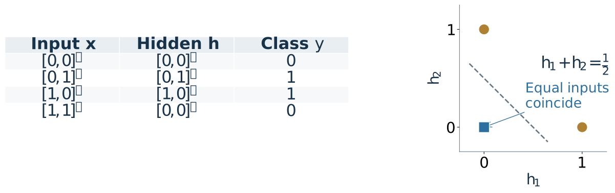
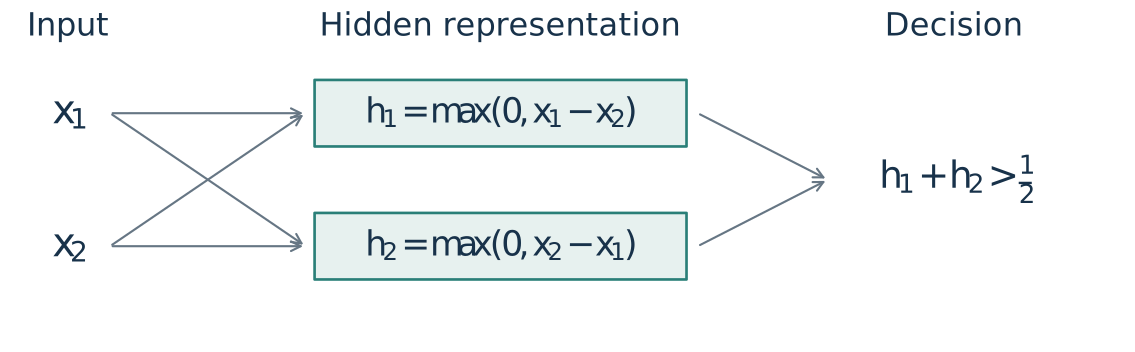
\[h_1=\max(0,x_1-x_2),\qquad h_2=\max(0,x_2-x_1).\]

\[h_1+h_2=|x_1-x_2|,\qquad \widehat y=\mathbb 1\{h_1+h_2>\tfrac12\}.\]

A linear decision in the hidden features solves the nonlinear input-space task.

About four minutes; work all four inputs using the arrows/table in the figure. Equal regions produce [0,0]; the two mismatch directions produce [1,0] and [0,1]. Hidden means an intermediate computed value, not an extra observed label. The sum is an affine readout of nonlinear features. These hand-set weights establish representability only; they do not demonstrate successful training or generalization. Later training must fit the feature map and the readout together. [Sources] source:d2l-multilayer-perceptrons, section5.1.1.2. Original exact construction.

A hidden layer collects several computed features into a vector

\[\boldsymbol{h}=[h_1,\ldots,h_m]^{\mathsf T}\in\mathbb R^m.\]

Each hidden unit has its own weights and bias; all see the same input.

The readout combines the resulting features.

About two minutes. The diagram specializes to the two-unit example, with the two formulas inside their nodes so edges do not become an uninterpretable hairball. Generalize the number of hidden units to m. The dashed conceptual separation is representation versus readout, not two separately fitted models. A dense layer allows every input-to-hidden connection even though a fitted weight could be zero. [Sources] source:d2l-multilayer-perceptrons, section5.1.1.2.

Stack the neuron weights to obtain one matrix expression

Each row of \(W\) is one neuron’s \(\boldsymbol w_j^{\mathsf T}\):

\[\boldsymbol h=\phi(W\boldsymbol x+\boldsymbol b),\qquad W\in\mathbb R^{m\times d},\quad \boldsymbol b\in\mathbb R^m.\]

Apply \(\phi\) separately to each feature.

For our two-region example:

\[W=\begin{bmatrix}1&-1\\-1&1\end{bmatrix},\quad \boldsymbol b=\begin{bmatrix}0\\0\end{bmatrix},\quad \boldsymbol h=\phi\!\left(\begin{bmatrix}x_1-x_2\\x_2-x_1\end{bmatrix}\right).\]

About two minutes. One observation is a column vector. Map each row to the neuron from the preceding diagram, rather than introducing a second orientation convention. Phi of a vector means elementwise ReLU; it is not matrix multiplication. Generic W and b are trainable, whereas the displayed example is an explicitly constructed setting. [Sources] source:d2l-multilayer-perceptrons, section5.1.1.3; translated to the course’s column-observation convention.