Learning Nonlinear Representations (continued)

ECE 57000 — October 14, 2026

David I. Inouye

Last time: nonlinear features made the mismatch task separable

• Fitting the training objective and generalizing to new examples are different goals.
• One linear score cannot express XOR; two ReLU units can construct useful features.
• A hidden layer computes \(\boldsymbol h=\phi(W\boldsymbol x+\boldsymbol b)\).

Today: revisit that toy construction, then build a multilayer perceptron and learn how its parameters receive gradients.

About one minute. Instructor-reported October 9 boundary: original slide 29 / runway +2, “Stack the neuron weights to obtain one matrix expression.” At the instructor’s request, begin review at original slide 27, then repeat the hidden-layer vector and matrix form before new material. Recording download and the remaining freeze/deploy work are paused; manual boundary and previous deck are preserved privately. This local deck is not authorized for publication. The core now gives a concise backpropagation overview with one worked example. The runway develops batch training and diagnostics; explicit matrix-gradient derivations have been removed at the instructor’s request. Section 3–4 previews remain orientation only.

Learned features expand what the model can represent

Arc 5 · Section 1 of 4

1. Representation: build nonlinear features ← this section
2. Training: learn the parameters
3. Image structure: design convolutional layers
4. Evaluation: test the architectural assumptions

Guiding question: Can learned features improve product-image classification?

Product images → XOR and ReLU → multilayer perceptrons → held-out evidence.

30-second orientation. The current class resumes this section at the toy construction; the canonical topic begins with the real-image task.

Two directional responses create a useful hidden representation

\[h_1=\max(0,x_1-x_2),\qquad h_2=\max(0,x_2-x_1).\]

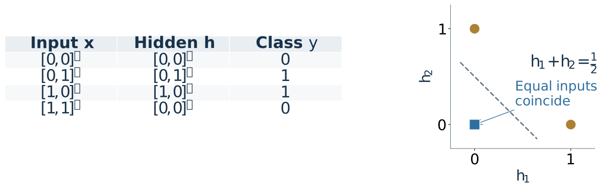
\[h_1+h_2=|x_1-x_2|,\qquad \widehat y=\mathbb 1\{h_1+h_2>\tfrac12\}.\]

A linear decision in the hidden features solves the nonlinear input-space task.

About four minutes; work all four inputs using the arrows/table in the figure. Equal regions produce [0,0]; the two mismatch directions produce [1,0] and [0,1]. Hidden means an intermediate computed value, not an extra observed label. The sum is a linear output layer of nonlinear features. These hand-set weights establish representability only; they do not demonstrate successful training or generalization. Later training must fit the feature map and the output layer together. [Sources] source:d2l-multilayer-perceptrons, section5.1.1.2. Original exact construction.

A hidden layer collects several computed features into a vector

\[\boldsymbol{h}=[h_1,\ldots,h_m]^{\mathsf T}\in\mathbb R^m.\]

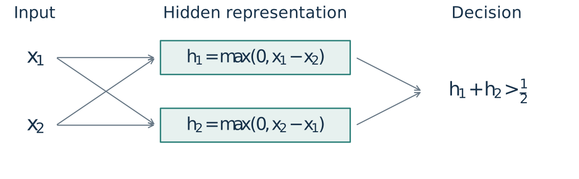
Each hidden unit has its own weights and bias; all see the same input.

The output layer combines the resulting features.

About two minutes. The diagram specializes to the two-unit example, with the two formulas inside their nodes so edges do not become an uninterpretable hairball. Generalize the number of hidden units to m. The dashed conceptual separation is representation versus output layer, not two separately fitted models. A dense layer allows every input-to-hidden connection even though a fitted weight could be zero. [Sources] source:d2l-multilayer-perceptrons, section5.1.1.2.

Stack the neuron weights to obtain one matrix expression

Each row of \(W\) is one neuron’s \(\boldsymbol w_j^{\mathsf T}\):

\[\boldsymbol h=\phi(W\boldsymbol x+\boldsymbol b),\qquad W\in\mathbb R^{m\times d},\quad \boldsymbol b\in\mathbb R^m.\]

Apply \(\phi\) separately to each feature.

For our two-region example:

\[W=\begin{bmatrix}1&-1\\-1&1\end{bmatrix},\quad \boldsymbol b=\begin{bmatrix}0\\0\end{bmatrix},\quad \boldsymbol h=\phi\!\left(\begin{bmatrix}x_1-x_2\\x_2-x_1\end{bmatrix}\right).\]

About two minutes. One observation is a column vector. Map each row to the neuron from the preceding diagram, rather than introducing a second orientation convention. Phi of a vector means elementwise ReLU; it is not matrix multiplication. Generic W and b are trainable, whereas the displayed example is an explicitly constructed setting. [Sources] source:d2l-multilayer-perceptrons, section5.1.1.3; translated to the course’s column-observation convention.

Dimensions account for every trainable parameter

One Fashion-MNIST image: \(784\) pixel features → \(64\) hidden units → \(10\) class scores.

\[\boldsymbol h=\operatorname{ReLU}(W\boldsymbol x+\boldsymbol b),\qquad \boldsymbol s=V\boldsymbol h+\boldsymbol c.\]

Layer	Weight matrix	Bias vector	Trainable parameters
Hidden layer	\(W:\ 64\times784\)	\(\boldsymbol b:\ 64\times1\)	\(64\cdot784+64=50{,}240\)
Output layer	\(V:\ 10\times64\)	\(\boldsymbol c:\ 10\times1\)	\(10\cdot64+10=650\)

Total: \(50{,}240+650=50{,}890\) trainable parameters.

Activations: \(\boldsymbol x\in\mathbb R^{784}\), \(\boldsymbol h\in\mathbb R^{64}\), \(\boldsymbol s,\boldsymbol p\in\mathbb R^{10}\). Softmax converts scores \(\boldsymbol s\) to probabilities \(\boldsymbol p\) and adds no parameters.

About two minutes. [Sources] source:fashion-mnist; source:d2l-multilayer-perceptrons. These are the exact dimensions of the product-image experiment. One observation is a column vector, with no batch axis yet. W,b,V,c are all the trainable parameters; inputs, activations, scores, and probabilities are computed values, not additional parameters. ReLU and softmax have no trainable parameters. Fixed-order flattening preserves pixel values but a dense layer does not enforce spatial locality or weight sharing.

The output layer maps learned features to multiclass probabilities

For the product images, let \(\boldsymbol h\in\mathbb R^{64}\) and compute

\[\boldsymbol s=V\boldsymbol h+\boldsymbol c,\qquad V\in\mathbb R^{10\times64},\quad\boldsymbol c\in\mathbb R^{10}.\]

Reuse softmax to normalize the ten scores into class probabilities:

\[p_c=\frac{\exp(s_c)}{\sum_{j=1}^{10}\exp(s_j)},\qquad c=1,\ldots,10.\]

For class labels \(y_i\), fit all parameters \(\boldsymbol\theta=(W,\boldsymbol b,V,\boldsymbol c)\) jointly using mean cross-entropy: \[J(\boldsymbol\theta)=-\frac1n\sum_i\log p_{i,y_i}.\]

About three minutes. Revisit the softmax/cross-entropy bridge introduced with the linear baseline. Only the learned input to the output layer changes: h replaces x. Binary sigmoid outputs one positive-class probability, whereas these ten mutually exclusive labels need one normalized distribution. Define p_c as the probability assigned to category c for this image and y as its class index. No one-hot encoding or softmax derivative is needed yet. Average this loss across training examples and add the selected L2 penalty. The linear baseline uses the same ten-score softmax output layer directly on x; the MLP inserts learned nonlinear h. The model is 784 -> 64 ReLU -> 10, with 50,890 parameters including the output layer. This is simpler to express using the matrix operations already taught; it is not claimed to use fewer parameters than every CNN. Numerical implementations subtract the largest score before exponentiating. [Sources] source:fashion-mnist; source:d2l-multilayer-perceptrons. Softmax is defined directly here as a normalized-exponential construction, not an unstated prerequisite.

Deeper models compose learned representations

\[\boldsymbol h^{(0)}=\boldsymbol x,\] \[\boldsymbol h^{(\ell)}=\phi_\ell\!\left(W_\ell\boldsymbol h^{(\ell-1)}+\boldsymbol b_\ell\right), \qquad \ell=1,\ldots,k.\]

\[\boldsymbol x\ \longrightarrow\ \boldsymbol h^{(1)}\ \longrightarrow\ \boldsymbol h^{(2)}\ \longrightarrow\ \text{prediction}.\]

Each layer transforms features produced by the previous layer.

An MLP—multilayer perceptron—uses dense layers with nonlinear hidden activations.

About two minutes. Superscripts index layers, not powers; k here counts hidden layers. If consecutive widths are m_(ell-1) and m_ell, W_ell has shape m_ell by m_(ell-1). ReLU can be used at every hidden layer, while the output layer depends on the task. A learned feature need not have a neat human label; do not promise an automatic edge-to-object hierarchy. This establishes the composition vocabulary before backpropagation or convolution. [Sources] source:d2l-multilayer-perceptrons, sections5.1.1.2–5.1.1.3.

Would extra linear layers solve the mismatch task?

A network has several hidden layers. Replace every hidden activation with the identity; compare the two final class scores.

Can it classify all four mismatch images correctly?

A. Yes, if the hidden layers are wide enough.

B. Yes, if gradient descent runs long enough.

C. No; the difference between its two final scores is still a linear score in the input.

C. Additional linear layers cannot supply the missing interaction.

Two-minute commitment-and-reveal question, including student thinking time. Width and optimization are plausible distractions; neither changes the represented function class here. Each final score is a linear score with a bias, so their difference is too; comparing them gives a linear decision boundary. Softmax preserves their ordering. Do not claim every deep linear parameterization has identical optimization or regularization behavior to fitting one matrix directly. Next slide proves the representational claim. [Sources] source:d2l-multilayer-perceptrons, section5.1.1.3.

Composing linear layers still gives one linear layer

A linear layer computes \(W\boldsymbol x+\boldsymbol b\) (technically affine when \(\boldsymbol b\ne\boldsymbol 0\)).

\(f(\boldsymbol x)\)

\(=\)

\(W_2(W_1\boldsymbol x+\boldsymbol b_1)+\boldsymbol b_2\)

(two linear layers)

\(\,\)

\(=\)

\(W_2W_1\boldsymbol x+W_2\boldsymbol b_1+\boldsymbol b_2\)

(distribute)

\(\,\)

\(=\)

\(A\boldsymbol x+\boldsymbol c\)

(\(A=W_2W_1\), \(\boldsymbol c=W_2\boldsymbol b_1+\boldsymbol b_2\))

Repeat this argument for any number of linear layers.

About three minutes. State compatible dimensions before expanding. The vector c here denotes the combined bias for a possibly vector-valued linear layer; it is the combined bias, not an extra trainable layer. A narrow hidden layer can restrict rank further, but never creates a nonlinear score. Keep the first complete equality visible initially and reveal one justified row at a time. [Sources] source:d2l-multilayer-perceptrons, section5.1.1.3; column-vector derivation.

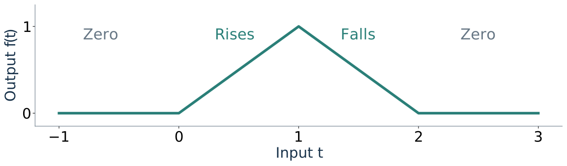
Nonlinear activations let simple pieces form a new shape

\[f(t)=\phi(t)-2\phi(t-1)+\phi(t-2),\qquad \phi(s)=\max(0,s).\]

The three ReLU units switch on at \(t=0,1,2\); the output weights are \(1,-2,1\).

Input interval	Substitute the active units
\(t\leq0\)	\(f(t)=0\)
\(0<t\leq1\)	\(f(t)=t\)
\(1<t\leq2\)	\(f(t)=t-2(t-1)=2-t\)
\(t>2\)	\(f(t)=t-2(t-1)+(t-2)=0\)

At \(t=1.5\): \(f(t)=1.5-2(0.5)+0=0.5\).

Each newly active unit changes the slope: \(0\to1\to-1\to0\). Three ReLU features plus a linear output layer create a shape no single linear layer can express.

About four minutes. Original analytic example. Read the table with the plot: inactive units contribute zero, and each active unit contributes its shifted input times its output weight. At each threshold the new unit changes the slope by its output weight. Walk through t=1.5 explicitly. For t below zero all units are off; from zero to one only the first is active; from one to two the first two are active; above two all three cancel. The graph is an exact calculation, not a fitted result. ReLU networks are piecewise linear, not necessarily smoothly curved. Nonlinearity expands what can be represented; it does not guarantee successful fitting. The formula is a one-hidden-layer instance of the same W,b,v,c architecture.

More expressive features still need held-out evidence

Question	Evidence needed
Can this architecture express a useful rule?	A construction or approximation argument
Did training find useful parameters?	Training objective and optimization diagnostics
Does the fitted predictor work on new examples?	Appropriate held-out evaluation

Choose width, depth, and regularization using validation data; reserve test data for final assessment.

Our four-image construction answers only the first question.

About two minutes. Revisit the Arc3/4 evaluation contract. Training improvements do not prove transfer; a wider model can express more but may need different amounts of data and computation. Learned hidden features do not remove the need to choose inputs, architecture, or splits. Do not introduce a universal monotonic width-to-test-error relationship. The tiny deterministic truth table has no measured generalization claim.

A small MLP makes fewer product-image errors in this experiment

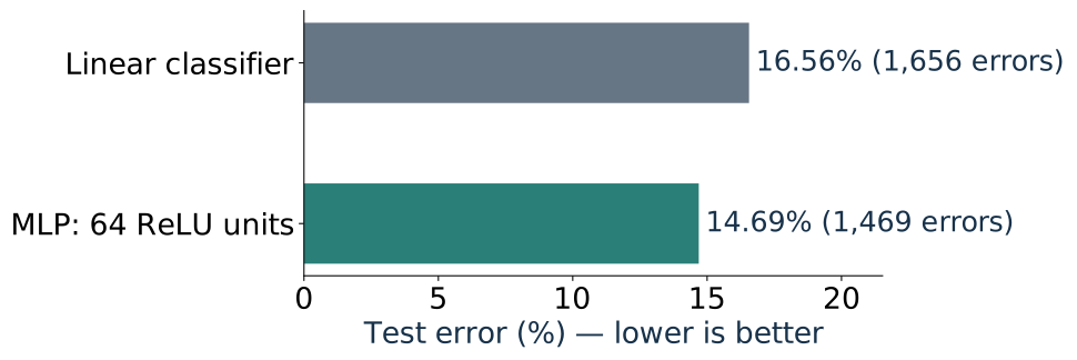
187 fewer errors on 10,000 test images. Same inputs and split; each model selected on validation data.

About two minutes. [Sources] source:fashion-mnist; source:fashion-mnist-train-images; source:fashion-mnist-train-labels; source:fashion-mnist-test-images; source:fashion-mnist-test-labels. Reproduced locally with lectures/scripts/arc5_fashion_mnist.py, recorded in fashion-mnist-results.json. The official 60,000-image training pool supplies a stratified 15,000-image subset with seed570, then 12,000 fit / 3,000 validation; 45,000 are unused. Test data are the full official 10,000 examples. Pixel scale is /255 for both. Linear model C candidates .01,.1,1,10; selected .1 (validation84.03%, test83.44%) converged in451 iterations. The C10 candidate reached its iteration cap and was not selected. MLP architecture is fixed 784->64ReLU->10softmax, Adam step .001, batch256, 60 epochs, alpha candidates .0001,.01,1; selected .01 (validation85.70%, test85.31%). All MLP fits hit the deliberately fixed epoch budget; no convergence claim. No refit, augmentation, test-driven tuning, favorable-seed search, CNN, or transformer comparison. Absolute error reduction1.87 percentage points; relative error reduction about11.3%. This modest gain is evidence for this fitted model on this split, not proof that all linear models have a nonzero irreducible error or that an MLP wins every dataset. Hand-set XOR features explained the mechanism; these features were learned from real training images.

The final loss must guide every layer’s parameters

Arc 5 · Section 2 of 4

1. Representation: build nonlinear features
2. Training: learn the parameters ← this section
3. Image structure: design convolutional layers
4. Evaluation: test the architectural assumptions

Guiding question: How can a final loss train earlier layers?

Gradient descent → atomic gradient rules → backpropagation → training diagnostics.

30-second orientation. This opens the training question. The next topic begins with gradient descent, explains reverse chain-rule evaluation, and uses one compact scalar example.

We still use gradient descent—but where do the gradients come from?

\[\boldsymbol\theta\leftarrow\boldsymbol\theta-\eta\nabla_{\boldsymbol\theta}J.\]

The parameters now sit inside a composition of many layers.

Backpropagation computes \(\nabla_{\boldsymbol\theta}J\) efficiently. Gradient descent (or Adam) uses those gradients to update the parameters.

Training loop: forward computation → backpropagation → parameter update.

About two minutes. Start from the already familiar optimizer. Backpropagation is the differentiation algorithm, not a replacement for gradient descent. For a batch objective, differentiate its mean loss. The next slides use a single-example scalar loss to isolate the mechanism. Original calculus exposition.

Backpropagation evaluates the chain rule from the loss backward

For \(a=f(\theta)\), \(b=g(a)\), and \(\ell=q(b)\):

\[\frac{\partial\ell}{\partial\theta} =\frac{\partial\ell}{\partial b}\, \frac{\partial b}{\partial a}\, \frac{\partial a}{\partial\theta}.\]

Forward: \(\theta\to a\to b\to\ell\); save the values needed by the derivatives.

Backward: start with \(\frac{\partial\ell}{\partial\ell}=1\), then compute

\[\frac{\partial\ell}{\partial b}=\frac{\partial q(b)}{\partial b},\qquad \frac{\partial\ell}{\partial a}=\frac{\partial\ell}{\partial b}\,\frac{\partial b}{\partial a},\qquad \frac{\partial\ell}{\partial\theta}=\frac{\partial\ell}{\partial a}\,\frac{\partial a}{\partial\theta}.\]

Same chain rule, reversed evaluation order. We need the forward output to evaluate the loss’s derivative, and saved intermediate values to evaluate the local derivatives.

About three minutes. The flipped aspect is the direction of sensitivity propagation, not an inverse function and not a new calculus identity. For squared loss \(q(b)=\tfrac12(b-y)^2\), \(\partial q(b)/\partial b=b-y\) depends on the computed prediction b; merely knowing the label is insufficient. Backward is seeded with one because the derivative of the scalar loss with respect to itself is one. The numeric loss value itself need not be stored if its derivative can be evaluated from the prediction and target. Values can alternatively be recomputed, trading computation for memory. Reverse accumulation shares intermediate sensitivities across parameters instead of redoing the whole chain for each parameter.

A few atomic operations supply the local gradient rules

Apply the reverse chain rule to each operation: incoming loss derivative × local derivative.

Forward operation	Send backward to its inputs	Forward values needed
\(q=a+b\)	\(\frac{\partial\ell}{\partial a}\mathrel{+}=\frac{\partial\ell}{\partial q}\), \(\frac{\partial\ell}{\partial b}\mathrel{+}=\frac{\partial\ell}{\partial q}\)	None
\(q=ab\)	\(\frac{\partial\ell}{\partial a}\mathrel{+}=b\frac{\partial\ell}{\partial q}\), \(\frac{\partial\ell}{\partial b}\mathrel{+}=a\frac{\partial\ell}{\partial q}\)	\(a,b\)
\(h=\operatorname{ReLU}(z)\)	\(\frac{\partial\ell}{\partial z}\mathrel{+}=\mathbb 1\{z>0\}\frac{\partial\ell}{\partial h}\)	Sign of \(z\) (or active mask)

Each rule multiplies the incoming sensitivity by a local derivative. The \(+=\) means add contributions if an input is used more than once.

About three minutes. All examples are scalar; matrix operations provide the corresponding vector rules. Explain accumulation in one sentence rather than a separate branching derivation. ReLU’s derivative is zero at negative inputs and one at positive inputs; at zero it is undefined and implementations choose a convention, commonly zero. Retaining the sign mask is sufficient for this backward rule. Multiplication needs the forward operands, showing why backward evaluation depends on saved values.

One forward pass supplies everything this backward pass needs

Toy scalar network: \(z=wx\), \(h=\operatorname{ReLU}(z)\), \(s=vh\), \(\ell=\tfrac12(s-y)^2\). Set \(x=2\), \(y=1\), \(w=1\), \(v=1\); omit biases to keep this example small.

1. Forward: compute and save

Value	Calculation
\(z\)	\(1\cdot2=2\)
\(h\)	\(\max(0,2)=2\)
\(s\)	\(1\cdot2=2\)
\(\ell\)	\(\tfrac12(2-1)^2=\tfrac12\)

Save \(h=2\) and the active ReLU mask.

2. Backward: start at the loss

Sensitivity / gradient	Calculation
\(\partial\ell/\partial s=s-y\)	\(2-1=1\)
\(\partial\ell/\partial v=(\partial\ell/\partial s) h\)	\(1\cdot2=2\) ← saved \(h\)
\(\partial\ell/\partial h=(\partial\ell/\partial s) v\)	\(1\cdot1=1\)
\(\partial\ell/\partial z=(\partial\ell/\partial h)\mathbb 1\{z>0\}\)	\(1\cdot1=1\) ← saved mask
\(\partial\ell/\partial w=(\partial\ell/\partial z) x\)	\(1\cdot2=2\)

Both weight gradients are \(2\). The optimizer can now update \(w\) and \(v\).

About four minutes. Original exact example, deliberately all on one slide. Read the left column top to bottom, then the right. The output weight gradient requires the numerical hidden activation h, not just its existence or shape. The ReLU backward rule requires knowing which branch was active in this forward pass. x and the old parameter values are also available. No update occurs midway through differentiation. The temporary scalar regression example explains the mechanism; the product-image model still uses softmax and cross-entropy. For eta=.01 the two weights become .98,.98; a fresh forward pass gives s=1.9208 and loss=.42393632. That optional arithmetic is not needed on the slide.

Libraries combine these rules to differentiate the whole network

1. Forward: record the operations and retain the values their backward rules need.
2. Backward: start at the scalar loss, apply local rules in reverse order, and sum contributions from shared paths.
3. Update: use the resulting gradient for every trainable parameter.

For our MLP, that includes \(W,\boldsymbol b,V,\boldsymbol c\).

We specify the model and loss; automatic differentiation organizes the chain rule.

About two minutes. Do not turn this into a matrix-gradient derivation. Matrix multiplication, elementwise activations, softmax, and loss operations have local backward rules, just like the scalar atoms. Backpropagation is reverse-mode automatic differentiation applied to the network graph. The optimizer is a separate step. Gradients use the current parameters and saved forward values; repeated training steps require fresh forward computations. No framework-specific API or version claims are needed.

Can an inactive ReLU receive a weight update from this example?

A hidden unit has \(z=-1\). There is no penalty term.

What does this example contribute to the gradient of its incoming weights?

A. Zero: the local ReLU derivative blocks this path.

B. Nonzero: a wrong prediction always changes every weight.

C. Undefined: ReLU has no derivative below zero.

A. Other examples may activate the unit; being inactive once does not make it permanently inactive.

Two-minute commitment-and-reveal discussion. This is the second live question in the current class after the linear-layer question. The nondifferentiable point is zero, not the negative half-line. Exclude penalty gradients; other examples or other uses of a shared parameter can still contribute. Reinforce the stored activation mask without a second worked derivation.

A training batch averages the example gradients

For a batch \(\mathcal B\) of \(B\) training examples:

\[J_{\mathcal B}(\boldsymbol\theta)=\frac1B\sum_{i\in\mathcal B}\ell_i(\boldsymbol\theta), \qquad \nabla J_{\mathcal B}=\frac1B\sum_{i\in\mathcal B}\nabla\ell_i.\]

One iteration: forward pass → average loss → backward pass → optimizer update.

An epoch processes the training set once. Clear old gradient accumulators before a new batch unless accumulation is intentional.

About two minutes. Reuse the earlier mini-batch and Adam discussion, not a new optimizer derivation. Conceptually sum per-example gradients; an implementation can batch matrix operations without materializing every example’s full gradient. For an explicitly chosen penalty lambda/2 times squared weight norms, add lambda W and lambda V; do not silently assume the library alpha convention matches this normalization. The displayed formula is the unpenalized data objective.

Finite differences can check a gradient implementation

Hold all other parameters fixed and perturb parameter \(\theta_j\):

\[g_j^{\mathrm{FD}}= \frac{J(\boldsymbol\theta+\epsilon\boldsymbol e_j)-J(\boldsymbol\theta-\epsilon\boldsymbol e_j)}{2\epsilon} \ \approx\ (\nabla J)_j.\]

For the scalar example, \(\epsilon=10^{-4}\) gives \(g_w^{\mathrm{FD}}\approx2\).

Use a tiny deterministic batch, double precision, and several small \(\epsilon\) values. Avoid perturbations that cross a ReLU kink.

This checks the derivative code, not the model’s generalization.

About three minutes. e_j here is a parameter-basis vector, introduced explicitly by the perturbation equation. For the scalar example at the original parameters, the central difference is exact up to floating point because the local loss is quadratic in w. Too small epsilon suffers cancellation and too large epsilon measures a finite-scale effect. Freeze randomness and use the same objective, reduction, and penalty on both sides. Compare absolute and relative discrepancies; do not divide only by a near-zero gradient. Numerical differentiation requires repeated loss evaluations and is a diagnostic, not the training method.