Training Neural Networks (continued)
ECE 57000 — October 16, 2026
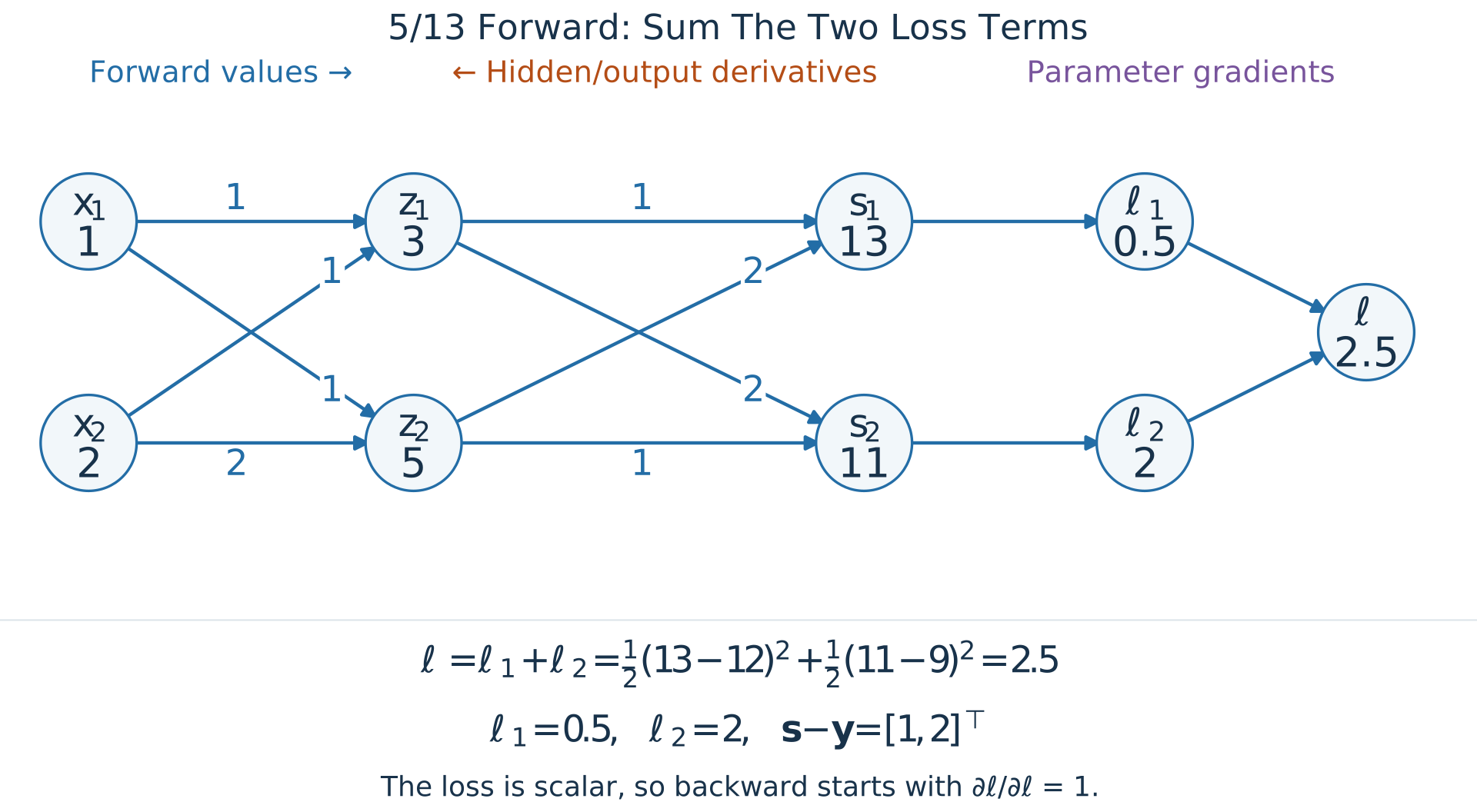
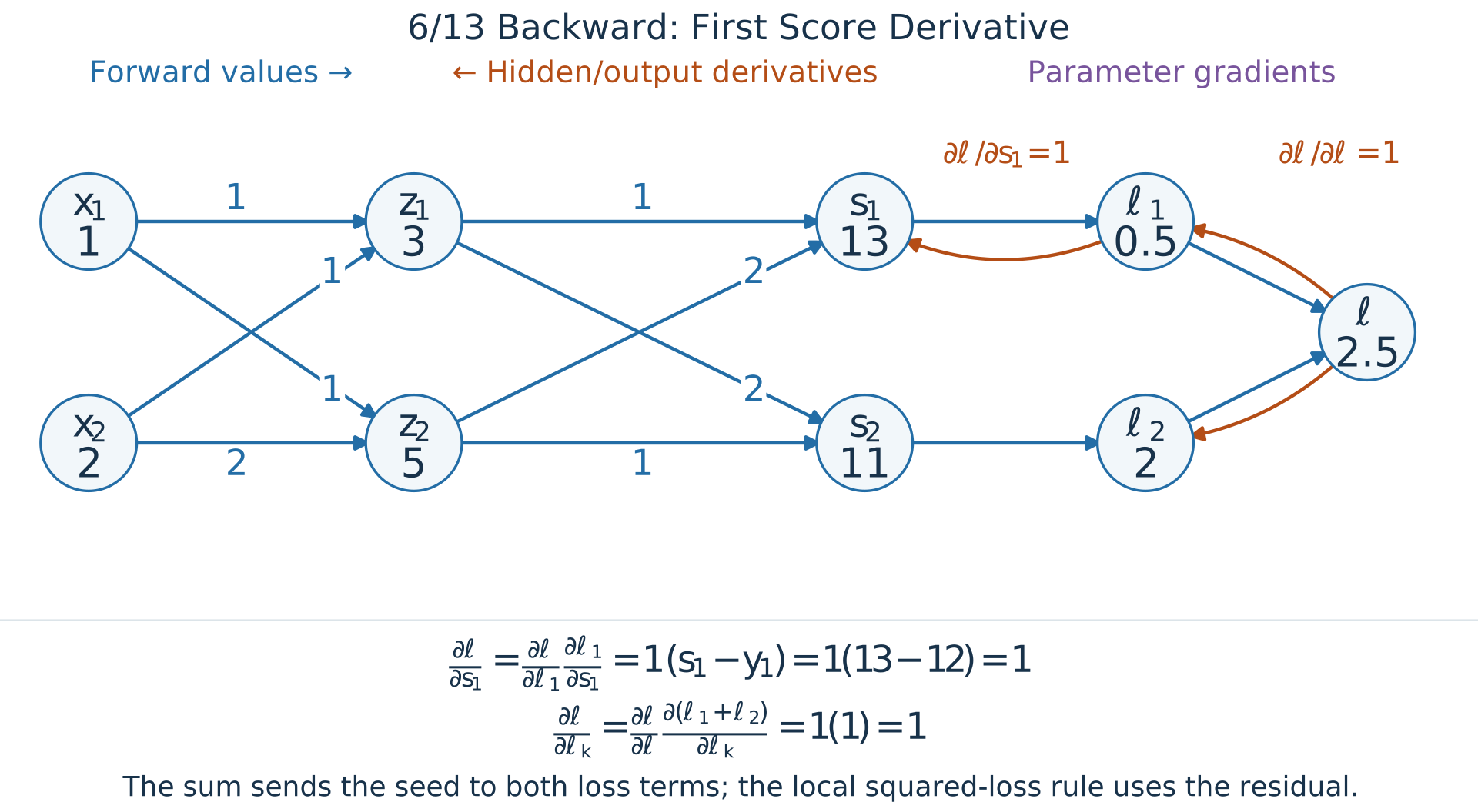
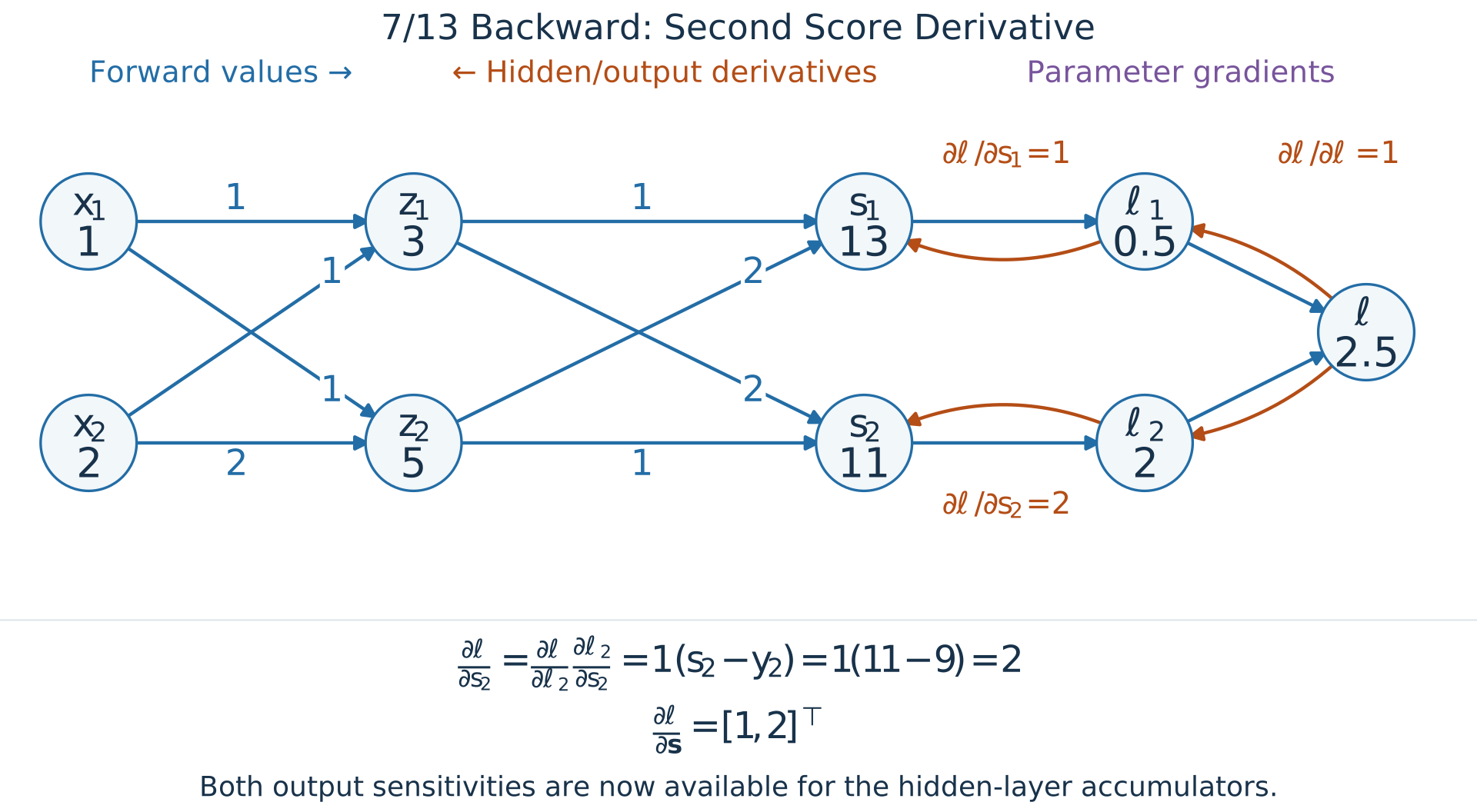
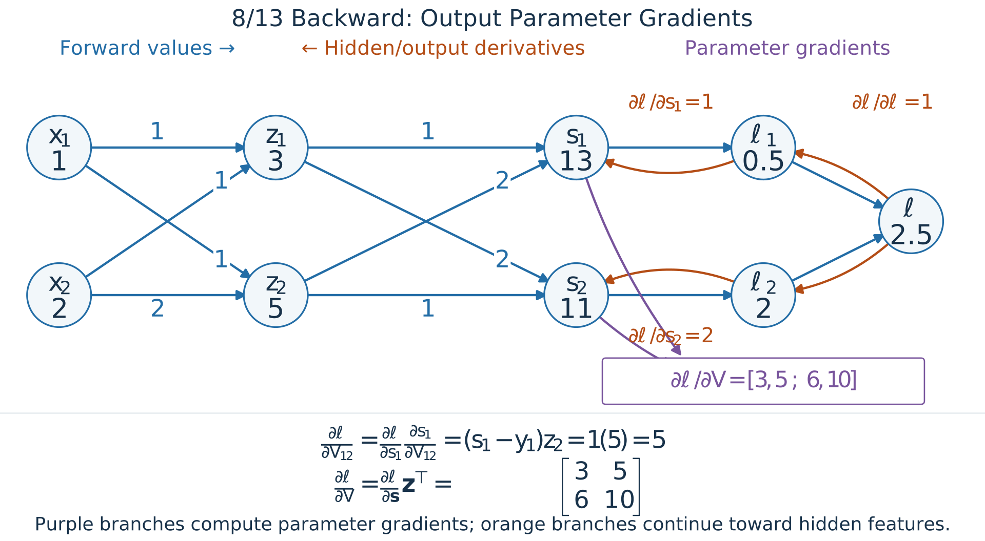
Backward computation sums paths at hidden features
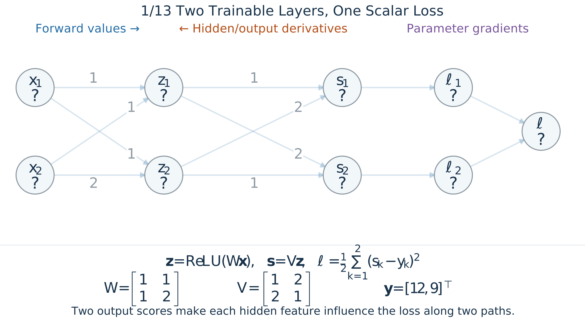
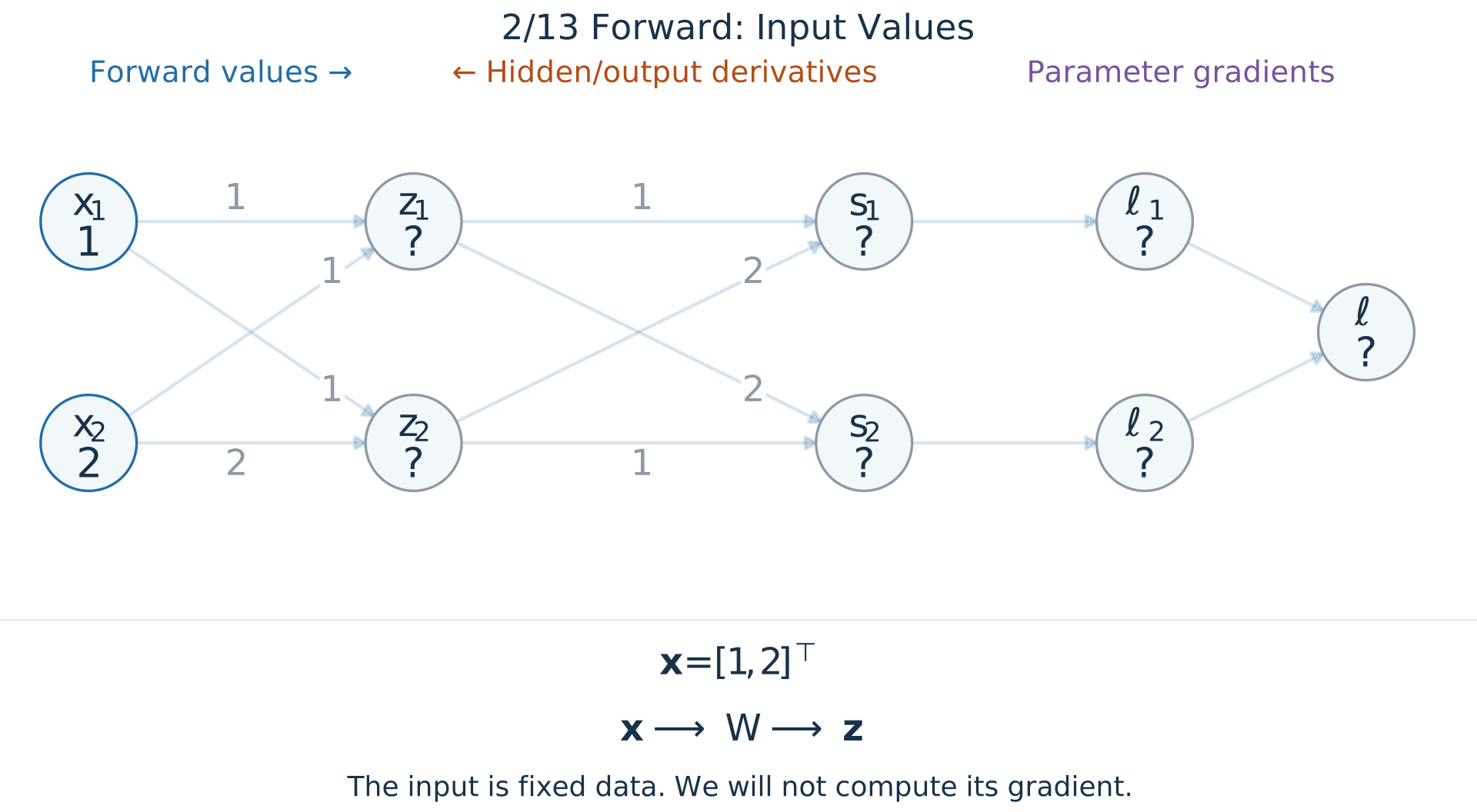
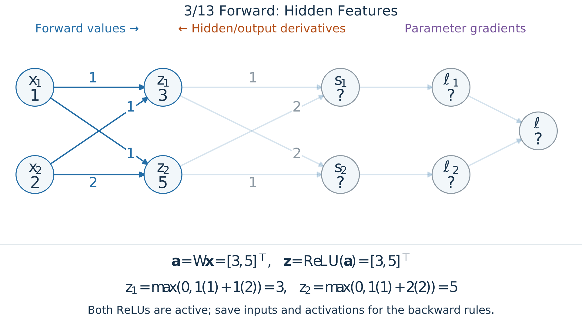
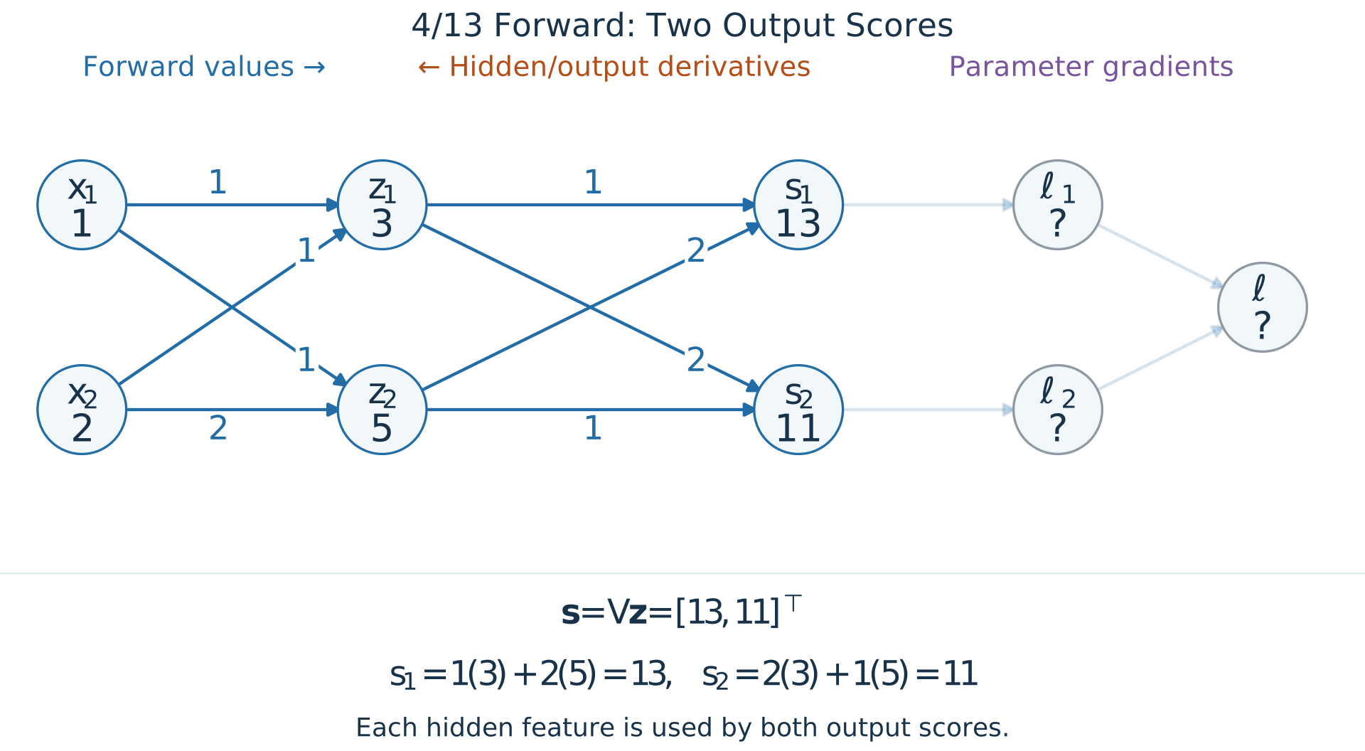
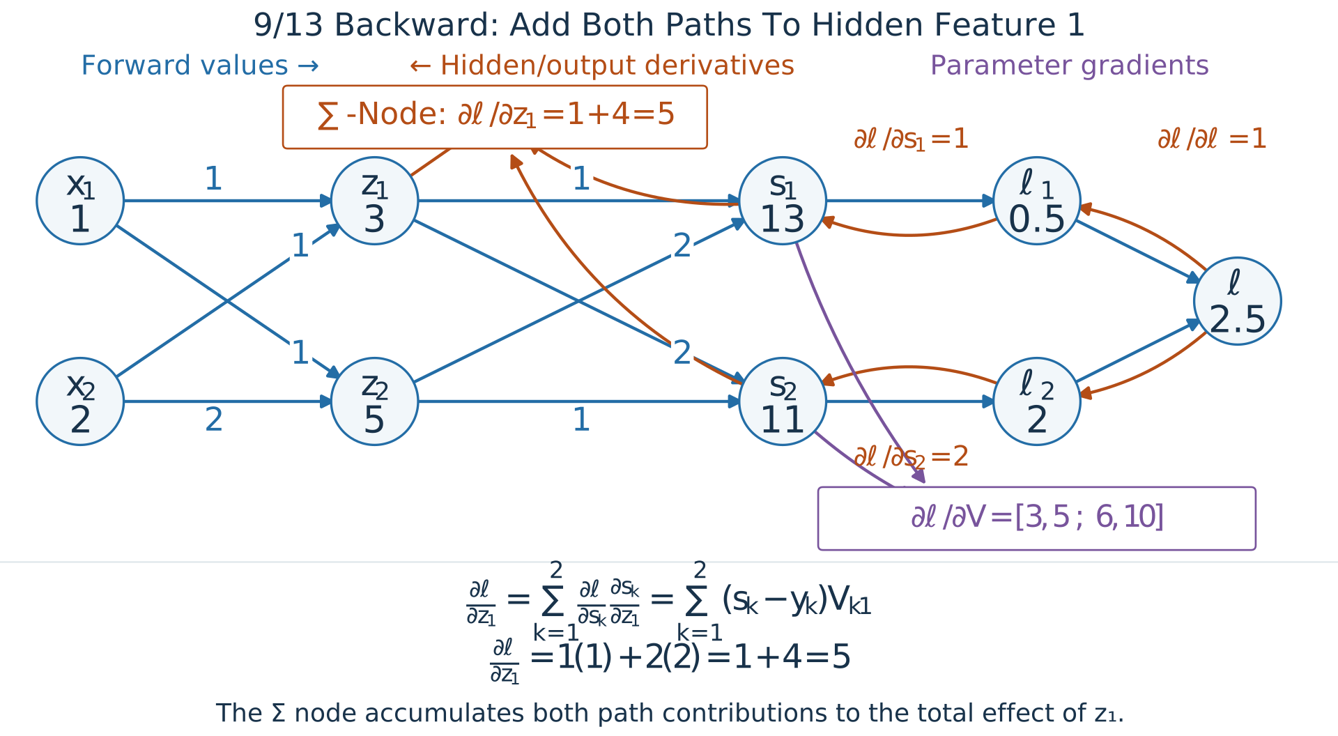
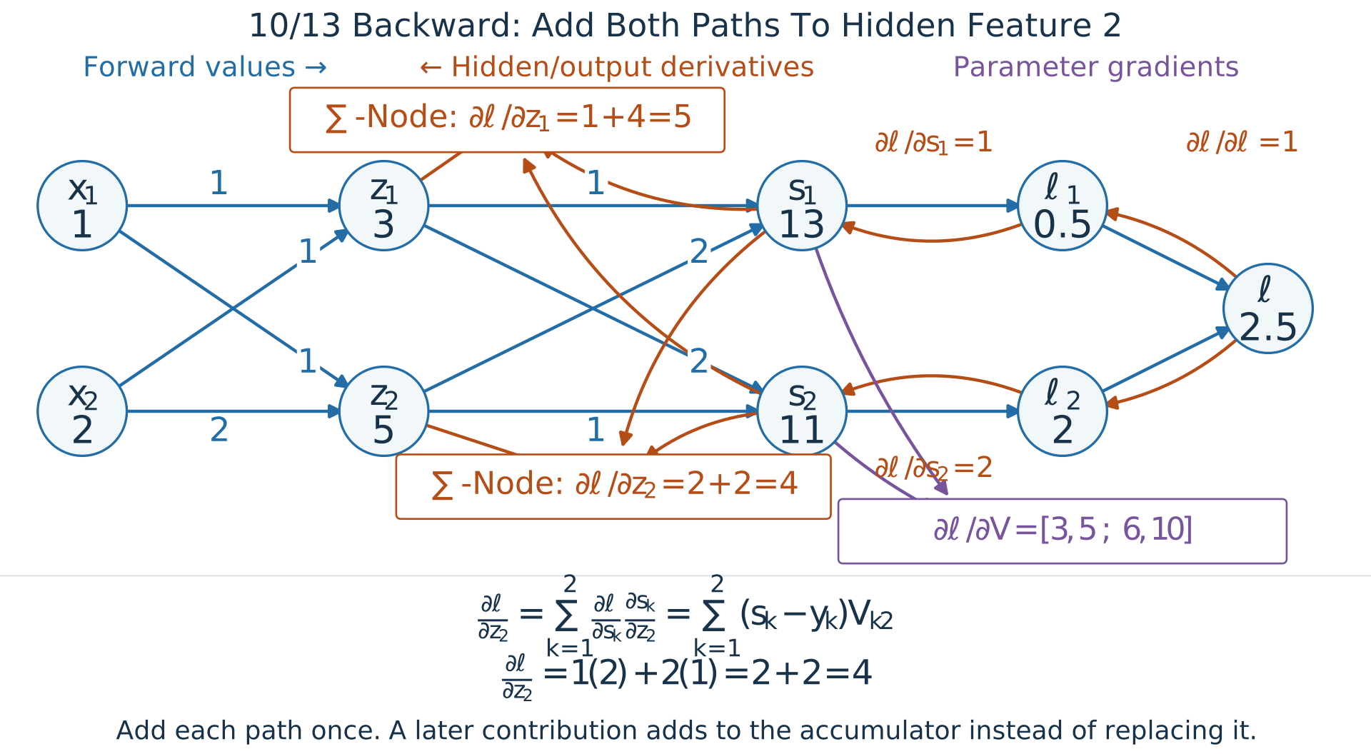
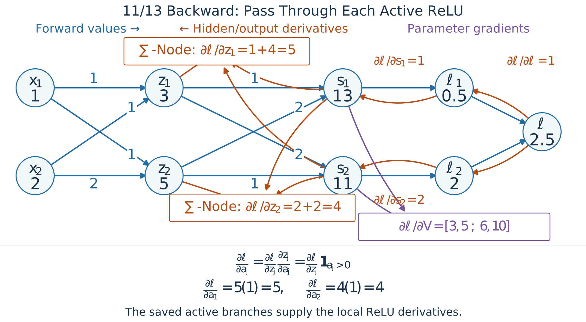
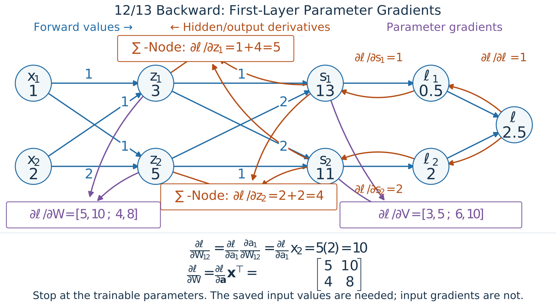
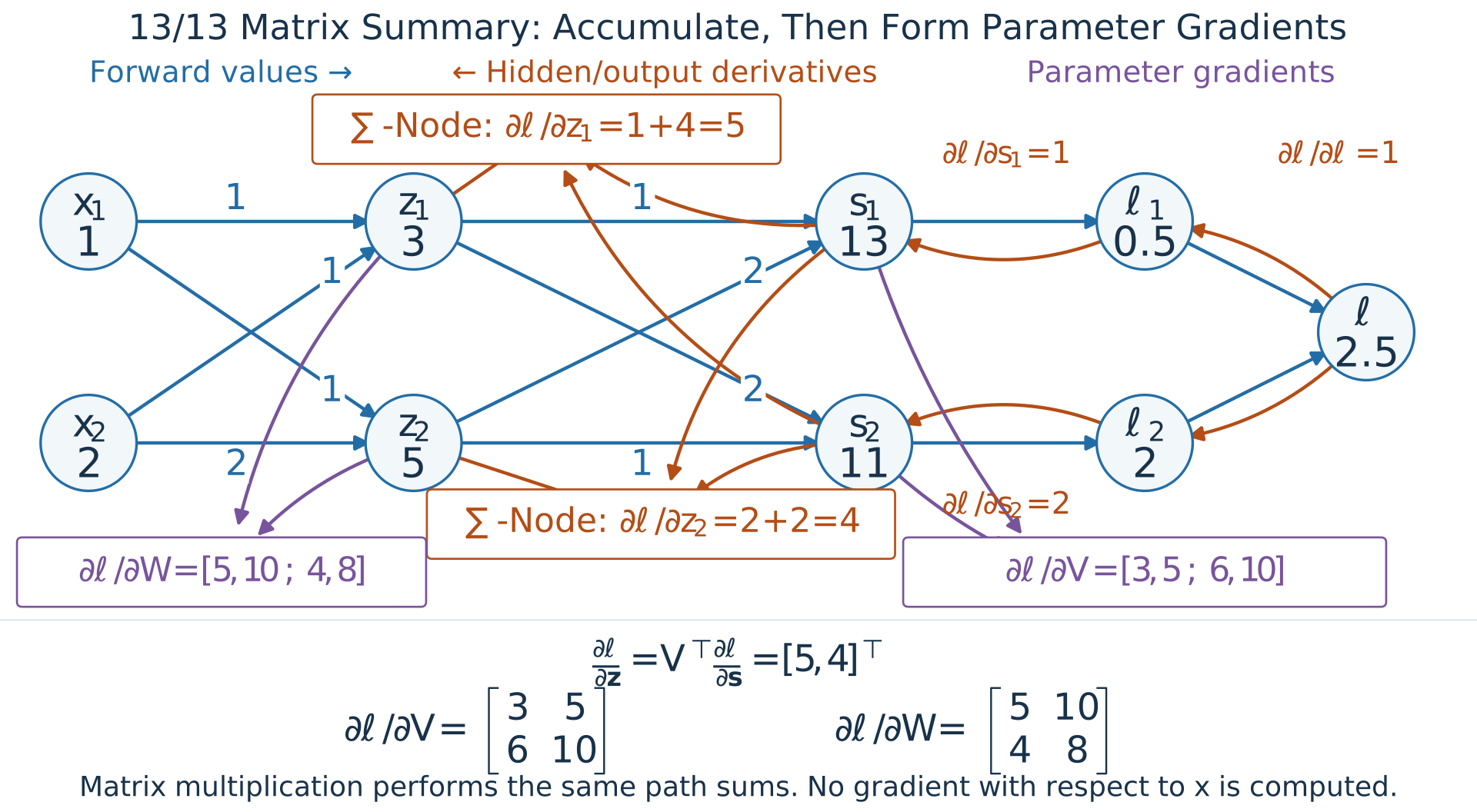
Backpropagation computes all parameter gradients efficiently
In 1D: \(\displaystyle\frac{\partial J}{\partial\theta}\approx\frac{J(\theta+\epsilon)-J(\theta)}{\epsilon}\).
One objective evaluation takes 1 second. Reuse the unperturbed value \(J(\boldsymbol\theta)\).
Finite differences: about how long for 10,000 parameters?
A. 2 seconds
B. 100 seconds
C. 10,000 seconds
C: 10,000 parameters → about 10,000 seconds.
One new evaluation per parameter.
Backpropagation: how long for the same full gradient?
Assume backward ≈ forward cost.
A. 2 seconds
B. 100 seconds
C. 10,000 seconds
A: about 2 seconds for forward + backward.
One reverse pass reuses work for all parameters.
Implementation connects the graph to running code
Arc 5 · Implementation in PyTorch
- Autograd: inspect the scalar computation and its gradients.
- Training: assemble the image model, loss, and optimizer.
- Diagnostics: inspect what the training loop produces.
The preceding section explained backpropagation mathematically. Now we make each operation concrete.
requires_grad identifies which inputs need derivatives
For scalar \(b=f(\boldsymbol a)\), computing \(\nabla_{\boldsymbol a} b\) requires marking a with requires_grad=True.
import torch
x = torch.tensor(2.)
y = torch.tensor(1.)
w = torch.tensor(1., requires_grad=True)
v = torch.tensor(1., requires_grad=True)
print(x.requires_grad, w.requires_grad, w.grad)
Output:
Mark the variable in the subscript of \(\nabla\)—or the denominator of \(\partial b/\partial a\) for scalars.
Here w and v are the trainable leaves. Their .grad fields will hold the weight derivatives after backward.
The forward pass builds values and a backward graph
print("Before computation, w.grad_fn:", w.grad_fn)
z = w * x
print("After computation, z.grad_fn:", type(z.grad_fn).__name__)
h = torch.relu(z)
s = v * h
r = s - y
loss = 0.5 * r.square()
print(z.item(), h.item(), s.item(), loss.item())
Output:
Forward values: \(w,x\to z\to h\); then \(v,h\to s\to r\to\ell\).
Backward graph: w is a leaf with no producing operation. Multiplying it creates z with a .grad_fn linking to that operation.
requires_grad=True enables tracking; the forward computation creates the graph.
Backward rules need selected forward values
For our scalar example:
| Operation | A value its backward rule needs | Here |
|---|---|---|
| \(z=wx\) | \(x\) to obtain \(\partial\ell/\partial w\) | \(2\) |
| \(h=\operatorname{ReLU}(z)\) | Which inputs were positive | Active |
| \(s=vh\) | \(h\) for \(v\)’s derivative; \(v\) for \(h\)’s | \(2\), \(1\) |
| \(\ell=\tfrac12 r^2\) | Residual \(r\) | \(1\) |
Saved forward values are not gradients. They let backward evaluate the local derivative rules.
We can observe what autograd saves for backward
saved = []
def pack(t):
    saved.append(t.detach().clone())  # snapshot for inspection
    return t.detach()                # value kept for backward

def unpack(t):
    return t

with torch.autograd.graph.saved_tensors_hooks(pack, unpack):
    loss = 0.5 * (v * torch.relu(w * x) - y).square()
print([t.item() for t in saved])
Output:
These values supply the multiplication, ReLU, and squared-loss backward rules.
One backward() computes both weight gradients
print("Before backward:", w.grad, v.grad)
loss.backward()
print("After backward:", w.grad.item(), v.grad.item())
print("Weights:", w.item(), v.item())
Output:
Backward starts at the scalar loss, follows the recorded graph, and adds contributions into the trainable leaves’ .grad fields.
The weights have not changed. Ordinary backward releases saved values; recompute forward for the next batch or updated weights.
What does .grad contain on the second iteration?
a = torch.tensor(1., requires_grad=True)
for iteration in range(2):
    b = a.square()
    b.backward()
    print(iteration + 1, a.grad.item())
Output after iteration 1:
What value of a.grad.item() will iteration 2 print?
A. \(2.0\) B. \(4.0\) C. \(0.0\)
zero_grad() begins a new gradient accumulation
def objective():
    return 0.5 * (v * torch.relu(w * x) - y).square()

optimizer = torch.optim.SGD([w, v], lr=0.1)
optimizer.zero_grad()
print("After reset:", w.grad)
loss = objective()
loss.backward()
print("After backward:", w.grad.item())
Output:
zero_grad() clears the previous accumulated gradients.
It resets gradients, not parameter values. Clear before each independent batch’s backward pass.
step() uses the gradients to change the weights
print("Before: w, v =", round(w.item(), 2), round(v.item(), 2))
print("Before: loss =", round(loss.item(), 4))
optimizer.step()
with torch.no_grad():
    new_loss = objective()
print("After:  w, v =", round(w.item(), 2), round(v.item(), 2))
print("After:  loss =", round(new_loss.item(), 4))
Output:
Here \(w,v: 1\to 1-0.1(2)=0.8\), and loss decreases from \(0.5\) to \(0.0392\).
no_grad() skips recording this evaluation; the next training forward pass records again.
The same operations train the product-image MLP
Implementation · From two scalar weights to 50,890 parameters
Data batch → model → scalar loss → backward → optimizer step.
Now assemble the complete loop, including validation.
A dataset provides examples; a loader assembles batches
from torch.utils.data import DataLoader, TensorDataset
# X_train: float32 [12000, 1, 28, 28], pixels in [0, 1]
# y_train: int64 [12000], class indices 0,...,9
train_dataset = TensorDataset(X_train, y_train)
train_loader = DataLoader(
    train_dataset, batch_size=64, shuffle=True)
val_loader = DataLoader(
    TensorDataset(X_val, y_val), batch_size=256)
xb, yb = next(iter(train_loader))
print(xb.shape, yb.shape)
Output:
Dataset: train_dataset[i] returns one image–label pair; len(train_dataset) is the number of examples.
DataLoader: iterates over batches of those pairs, handling batch size and shuffling. Here next(iter(train_loader)) returns 64 examples.
nn.Module collects the model’s trainable parameters
from torch import nn
torch.manual_seed(570)
model = nn.Sequential(
    nn.Flatten(),
    nn.Linear(784, 64),
    nn.ReLU(),
    nn.Linear(64, 10))
print(sum(p.numel() for p in model.parameters()))
Output:
Batch shapes: [B, 1, 28, 28] → [B, 784] → [B, 64] → [B, 10].
model.parameters() collects the trainable weights and biases, already marked requires_grad=True.
Cross-entropy consumes scores before softmax
loss_fn = nn.CrossEntropyLoss()
logits = model(xb)       # [B, 10] unnormalized scores
loss = loss_fn(logits, yb)
print(loss.shape)
Output:
The loss combines log-softmax with the true class’s negative log probability, then averages over this batch.
Pass logits directly. Use logits.argmax(dim=1) to choose classes; softmax is only needed when displaying probabilities.
One batch needs four distinct training operations
optimizer = torch.optim.Adam(model.parameters(), lr=1e-3)
model.train()                        # set training mode only
optimizer.zero_grad(set_to_none=True)  # clear
loss = loss_fn(model(xb), yb)          # forward
loss.backward()                       # differentiate
optimizer.step()                      # update
model.train() only sets training mode for layers such as dropout and batch normalization. It does not compute gradients or update weights.
| Operation | Changes |
|---|---|
zero_grad() |
Stored parameter gradients |
Forward and backward() |
Activations, graph, then gradients |
step() |
Parameter values and optimizer state |
An epoch repeats the update for every training batch
def train_one_epoch(model, loader, loss_fn, optimizer):
    model.train()  # set training mode only
    total_loss, count = 0.0, 0
    for xb, yb in loader:
        optimizer.zero_grad(set_to_none=True)
        loss = loss_fn(model(xb), yb)
        loss.backward()
        optimizer.step()
        total_loss += loss.item() * len(yb)
        count += len(yb)
    return total_loss / count
Multiply each batch’s mean loss by its size so a short final batch receives the correct weight.
This records the losses observed during training, as the weights change.
Validation measures predictions without updating the model
@torch.no_grad()
def evaluate(model, loader, loss_fn):
    model.eval()  # set evaluation mode only
    total_loss, correct, count = 0.0, 0, 0
    for xb, yb in loader:
        logits = model(xb)
        total_loss += loss_fn(logits, yb).item() * len(yb)
        correct += (logits.argmax(1) == yb).sum().item()
        count += len(yb)
    return total_loss / count, correct / count
train() / eval() only select layer behavior—important for dropout and batch normalization. Neither runs training or evaluation.
no_grad() disables graph recording. Mode and gradient tracking are separate.
The complete loop joins learning and held-out evaluation
optimizer = torch.optim.Adam(model.parameters(), lr=1e-3)
for epoch in range(5):
    train_loss = train_one_epoch(
        model, train_loader, loss_fn, optimizer)
    val_loss, val_acc = evaluate(model, val_loader, loss_fn)
    print(f"{epoch + 1}: train={train_loss:.3f}, "
          f"val={val_loss:.3f}, accuracy={val_acc:.1%}")
Output:
1: train=0.843, val=0.602, accuracy=79.6%
2: train=0.538, val=0.525, accuracy=82.2%
3: train=0.489, val=0.498, accuracy=83.1%
4: train=0.448, val=0.482, accuracy=83.6%
5: train=0.420, val=0.464, accuracy=84.1%
Model → loss → gradient → update → validation. The functions above now form one complete training loop.
Five epochs are a demonstration budget; validation guides later choices. Keep the test set untouched.
detach() keeps the values but cuts the gradient path
u = torch.tensor(1., requires_grad=True)
q = torch.tensor(1., requires_grad=True)
hidden = torch.relu(u * 2.).detach()
loss = 0.5 * (q * hidden - 1.).square()
loss.backward()
print(hidden.item(), hidden.requires_grad)
print(u.grad, q.grad.item())
Output:
The detached tensor has the same values, treated as constants for this backward pass. The loss trains q, but not u through this path.
Useful: train a new prediction layer on fixed features, or compute diagnostics from predictions without extending their training graph.
Store diagnostic values without keeping their training graphs
loss_history, score_history = [], []
logits = model(xb)
loss = loss_fn(logits, yb)
loss_history.append(loss.item())
score_history.append(logits.detach().cpu().clone())
print(type(loss_history[-1]).__name__)
print(score_history[-1].requires_grad)
loss.backward()
Output:
Use .item() for a scalar loss; store detached scores for later plots or evaluation metrics. The original loss still supports backward.
Storing loss or logits directly keeps references to their graphs. Logging should keep the numbers, not their training history.
Initialization is part of the training recipe
- PyTorch provides useful defaults: standard layers initialize their parameters when constructed;
nn.Linearscales its initial values with the input width. - Match the method you reproduce: follow a paper’s specified initialization, including its scale, distribution, and bias settings. Defaults may differ.
- Initialization can materially change training and the final model. Record the strategy and random seed; use multiple seeds when comparing results.
torch.nn.init provides strategies such as Xavier and Kaiming initialization. Choose for the architecture and activation; do not replace a paper’s recipe blindly.