Convolutions and Image Architectures

ECE 57000 — October 21, 2026

David I. Inouye

Convolution combines local connections and shared parameters

• A filter spans all input channels; each learned filter produces one output channel.
• Kernel size, padding, and stride determine spatial output size; filter count determines channel count.
• Stack convolutions with nonlinearities to expand the receptive field; reuse the same training loop.

Today: finish and evaluate the simple CNN, then read ResNet and U-Net architectures.

About two minutes. Recap October 19. Repeat the final small CNN slide for continuity, then use the pixel-permutation question to motivate empirical architectural comparison. Keep parameter memory distinct from computational cost.

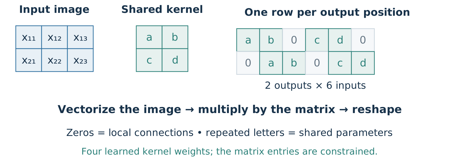
A convolution is a sparse matrix with shared entries

\[\operatorname{vec}(Y)=A_K\operatorname{vec}(X),\qquad A_K=\begin{bmatrix}a&b&0&c&d&0\\0&a&b&0&c&d\end{bmatrix}.\]

About three minutes. Formalize the explanation given orally on October 19. X is a 2×3 matrix, K is a 2×2 kernel, and Y is 1×2; vec stacks rows into a column here. Explicit row-major order: [x11,x12,x13,x21,x22,x23]^T. First row selects the left patch, second row the right patch. This uses PyTorch cross-correlation convention: no kernel flip. Four free weights, not twelve independent matrix parameters. A shared bias adds b_0 times the all-ones vector; omitted here to isolate the linear operator, with no activation. This is a conceptual matrix, not a recommendation to materialize it. Zeros express locality; tying expresses reuse. The numerical example X=[[1,2,3],[4,5,6]], K=[[1,2],[3,4]] gives [37,47]. Later reuse exactly this A_K to explain its transpose. [Sources] source:pytorch-conv2d-2-7.

A small CNN changes the model but reuses the training loop

cnn = nn.Sequential(
    nn.Conv2d(1, 8, 3, padding=1),
    nn.ReLU(),
    nn.Conv2d(8, 16, 3, stride=2, padding=1),
    nn.ReLU(),
    nn.Flatten(),
    nn.Linear(16 * 14 * 14, 10))
a = torch.zeros(64, 1, 28, 28)
for layer in cnn:
    a = layer(a)
    print(type(layer).__name__, tuple(a.shape))

Output:

Conv2d (64, 8, 28, 28)
ReLU (64, 8, 28, 28)
Conv2d (64, 16, 14, 14)
ReLU (64, 16, 14, 14)
Flatten (64, 3136)
Linear (64, 10)

About four minutes. Every line of output is captured from the verified model in arc5_convolution_figures.py. Zero inputs are only a shape probe, not training data. ReLU preserves shape, Flatten keeps the batch axis, and the final layer supplies ten logits for the same cross-entropy. To train this new model, construct its optimizer from cnn.parameters(), then pass cnn and that optimizer to the existing train_one_epoch and evaluate helpers. Do not reuse the old MLP’s optimizer. This model has 32,618 parameters; the following topic reports its fixed-protocol comparison. [Sources] source:pytorch-conv2d-2-7.

Keep the pixels, change their arrangement

Randomly permute pixel positions. Use the same permutation for every image, then retrain both models.

Which model’s architectural advantage would you expect to shrink?

A. MLP

B. CNN

C. Both equally

B. CNN. The information remains, but nearby entries no longer form local image patterns.

About three minutes including voting. Central emphasis: architecture helps by matching structure in the data, not by creating additional input information. This question follows the complete CNN and leads directly into evaluating its assumptions. B is the best prediction about the locality/shared-pattern advantage, not a guaranteed accuracy ranking. C is tempting because the shuffled image looks equally scrambled to a person; A may reflect the idea that an MLP cannot undo a shuffle. A fixed permutation loses no pixel information, and a fully connected first layer can absorb it by permuting its input weights. In contrast, convolution now ties local rules over arbitrary neighborhoods rather than nearby image locations. This does not prove every CNN must perform worse or that finite training gives exactly the same MLP accuracy. A different random permutation for each image would be a different experiment. We have not measured this intervention; the next section measures the original models and a separately defined translation stress. Do not turn this into a detour on permutation notation.

Convolution provides structure, not a guarantee of accuracy

• Locality: each output sees a patch, expanded by stacking layers.
• Sharing: the same filters are reused across positions.
• Shape control: filters choose channels; kernel, padding, and stride choose spatial sizes.

Next, compare CNN and MLP using the same data splits and a documented training/selection protocol.

The design is now explicit. Its benefit is an empirical question.

About one minute. Wrap the operation and shape intuitions before empirical architecture evaluation. Save the position/invariance distinction for the prediction question and counterexample in the next topic; do not preempt its reveal. The next topic measures these particular models under a fixed classroom protocol; do not generalize its result to every CNN. [Sources] source:pytorch-conv2d-2-7.

Testing Architectural Assumptions

Architectural assumptions need empirical evidence

Arc 5: CNN fundamentals → empirical evidence → ResNet classification → U-Net segmentation.

1. Compare: what changes under the same training recipe?
2. Stress: what happens when image position changes?
3. Decide: which conclusions does the evidence support?

Locality and sharing motivate the CNN. Now test what they buy us.

30-second orientation. Return from building a network to testing its assumptions, before reading two canonical architectures. Use this stable Compare → Stress → Decide structure for the controlled comparison, shifted validation condition, and conditional conclusion. All measured results come from the original fixed-protocol classroom experiment; do not infer a universal architecture ranking.

Compare architectures under one stated recipe

Keep fixed	Change
Same 12,000 training / 3,000 validation images	MLP: 784 → 64 → 10
Same batches, five epochs, Adam at \(10^{-3}\)	CNN: the two-convolution model just shown
Three seeds; use the final epoch of every run	Connections, parameter count, and computation

Equal epochs give equal data passes—not equal computation.

No augmentation, tuning, or test-set access in this comparison.

About three minutes. Original classroom experiment, arc5_architecture_comparison.py and comparison-results.json. The same archived split and pixel scaling are reused; training batch size is 64. Seeds 570, 571, 572 control initialization and an independent batch-order generator; the batch sequence matches between architectures for each seed. Both use standard layer initialization, but different architectures do not receive identical initial functions. Each run starts fresh; no best-seed or best-epoch selection. Equal optimizer settings are a transparent baseline, not individually optimized settings or a guarantee of equal optimization difficulty. Five epochs are not a convergence claim. This comparison estimates performance of these two complete recipes; it does not isolate weight sharing alone. Validation is deliberately used for exploration; the official test set is not loaded. [Sources] source:fashion-mnist; source:pytorch-optimization-tutorial.

This CNN improves validation accuracy under this recipe

Model	Mean accuracy	Range across three seeds
MLP	83.4%	83.0–83.7%
CNN	86.0%	85.7–86.3%

Same 3,000 validation images; five training epochs per run.

Supported: this CNN recipe performed better on this split.

Not established: every CNN beats every MLP, or the gap persists under equal compute.

About three minutes. Values are rounded from comparison-results.json: MLP 83.0333, 83.4333, 83.6667%; CNN 86.1667, 86.3, 85.6667%. Means are 83.3778 and 86.0444%, a 2.67 percentage-point difference. Seed ranges describe fitting randomness on one fixed split, not confidence intervals or sampling uncertainty. The two models differ in width, connectivity, sharing, depth, and parameter count; do not attribute the gap exclusively to convolution. These new five-epoch PyTorch runs are separate from both Friday’s demonstration and the earlier 60-epoch scikit-learn experiment. No test accuracy is claimed.

Fewer parameters can still require more computation

Complete model	Learned parameters	Multiply-accumulates per image
MLP	50,890	50,816
CNN	32,618	313,600

A convolution stores a filter once but applies it at many positions.

This CNN has about 36% fewer parameters and 6.2× as many multiply-accumulates.

About three minutes. Exact counts for the authored models. MLP parameters: 78464+64+6410+10=50,890; dense multiply-accumulates: 78464+6410=50,816. CNN parameters: (189+8)+(8169+16)+(313610+10)=32,618. CNN multiply-accumulates: 282889 + 14141689 + 3136*10 = 313,600. Counts exclude bias additions, activations, memory traffic, backward computation, and optimizer work. One multiply-accumulate is counted as one; it is sometimes counted as two floating-point operations. These are arithmetic counts, not a measured latency ratio. Hardware kernels and memory access affect runtime; activation memory is also distinct from parameter storage.

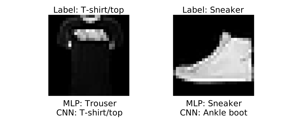
A better average can hide different mistakes

The CNN fixes one MLP error; the MLP gets another example right.

Inspect disagreements against the label before deciding which errors matter.

About two minutes. These are selected examples, not random or representative error samples. For seed 570, choose the first validation index where CNN is correct and MLP wrong (index 1), then the first with the opposite outcome (index 308). Selection rule was fixed in the experiment code. Labels and both predictions are generated from actual model outputs. The two examples demonstrate that a mean does not imply pointwise dominance; they do not establish class-specific reliability or error severity. In a real task, inspect labels and quantify errors relevant to the intended use before making a choice. [Sources] source:fashion-mnist.

Stress the assumption about position

Architecture evaluation · 2/3 Stress · Compare → Stress → Decide

30-second transition. Original validation favors one recipe. The convolution motivation also invoked patterns occurring at different positions. Test that claim by changing position while keeping the model fixed.

Predict what happens when the image moves

A CNN uses convolution, then flattening and a linear classifier.

Must shifting an image preserve its predicted class?

A. Yes, filters are shared

B. Only for one-pixel shifts

C. No, the classifier can use position

C. A pattern can move in the feature map; the classifier can weight positions differently.

About three minutes, optional runway question. A confuses shared local detection with invariant classification. B incorrectly assumes small shifts are inherently protected; stride can make one-pixel shifts especially consequential. C is a counterexample claim, not a prediction that every image must flip. Keep the architecture condition visible. Do not reveal this answer in the title or preceding divider. The next slide constructs the smallest example so the distinction is immediately concrete. Equivariance itself is qualified by boundaries and stride alignment. [Sources] source:pytorch-conv2d-2-7.

A shared filter can feed a position-sensitive decision

Use a size-one filter with weight 1 and bias 0. It copies each input value.

	Original	Shift right
Input and feature map	\([0,1,0]\)	\([0,0,1]\)
Class A score: middle entry	1	0
Class B score: right entry	0	1
Prediction	A	B

Same filter at every position; different class after a shift.

About two minutes. Original exact counterexample, verified with Conv1d and a fixed linear readout in the companion script. This is a schematic classifier, not a trained Fashion-MNIST result. The input content is moved without cropping the nonzero entry. The convolutional feature map moves with the input, but the flattened readout assigns different roles to its positions. This proves convolution alone does not guarantee invariant classification. Pooling/aggregation or augmentation may encourage invariance, but each has conditions and tradeoffs; do not imply they provide universal robustness.

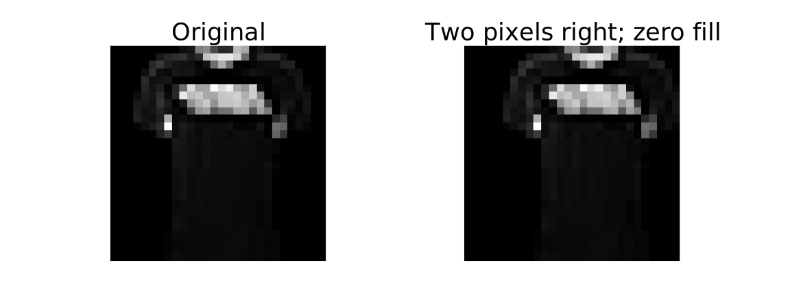
Define the shift before interpreting its score

Move each validation image two pixels right. Fill the left edge with zeros; discard the rightmost two columns. No wrapping.

Keep the original labels. This assumes the remaining image still supports the same category.

About two minutes. The illustrative image is the first stored disagreement example. Apply exactly this transformation to all 3,000 validation images without retraining either model or choosing a favorable seed. This is a separately labeled stress condition, not a replacement validation split or a new independent sample. Zero filling and clipping change pixels as well as position, so the resulting accuracy drop cannot be attributed solely to failure of translation equivariance. Retaining labels is plausible for this limited shift but requires scrutiny if informative parts are clipped. [Sources] source:fashion-mnist.

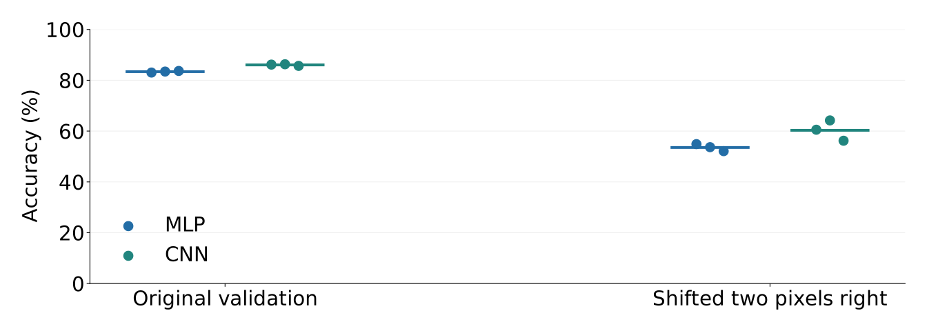
Both models lose accuracy on shifted images

Mean accuracy: MLP 83.4% → 53.5%; CNN 86.0% → 60.3%.

The CNN does better here, but its original validation accuracy does not establish shift robustness.

About three minutes. Each dot is one fixed seed; the short horizontal mark is its mean. Original and shifted images are paired; no retraining occurs. Means: MLP 83.3778→53.5444%; CNN 86.0444→60.3111%. Drops are about 29.8 and 25.7 percentage points. Three seeds are not three new datasets. Stride, positional readout, clipping, and absence of augmentation can all contribute; this experiment does not isolate their effects. One rightward shift does not characterize all perturbations, domains, or CNNs. Do not tune on this stress set and subsequently call it independent final evidence.

Choose a model for the conditions it must handle

Architecture evaluation · 3/3 Decide

Evidence so far	Decision it informs
Higher original validation accuracy	Candidate for similarly positioned images
Fewer parameters, more arithmetic	Check storage and runtime budgets separately
Large shifted-image accuracy loss	Investigate position variation before deployment

Compare → Stress → Decide: a single accuracy number cannot settle all three.

About three minutes. This is substantive synthesis, not a 30-second orientation: it asks students to connect results to a decision. If the deployment resembles original validation and these resource requirements fit, CNN is a reasonable candidate among these two recipes. If translations are common, neither original score is sufficient. Actual latency, activation memory, and relevant errors require additional measurement. Do not claim a particular model meets an unstated application threshold.

Architectural bias helps when its assumptions fit

• Assumption: local patterns recur; sharing is useful when that is true.
• Evidence: these two recipes favor the CNN on one split; both degrade under one shift.
• Next test: fix the recipe and selection rule, then evaluate on held-out data matching the intended conditions.

More expressive features, efficient gradients, and a working loop are necessary steps. They do not replace evidence about where the model will be used.

About three minutes. Close the simple comparison before introducing ResNet and U-Net as complete architectural examples. Limits of this comparison: one dataset/split, two small architectures, three initialization/batch-order seeds, five epochs, one optimizer recipe, and one artificial stress condition. No uncertainty over new dataset draws or converged-model ranking was established. All exploration used validation, not the official test set. The earlier scikit-learn study already reported official test results, so even a later test of this new recipe must disclose that prior dataset-level exposure; do not call the benchmark wholly untouched by the course. New independent application data are needed for a stronger deployment claim. Additional augmentation, tuning, or architectures would need an explicit selection protocol and fresh final evidence.

Image Classification with ResNet

A realistic classifier combines updates, normalization, and aggregation

Arc 5: CNN fundamentals → empirical evidence → ResNet classification → U-Net segmentation.

1. Update: refine a representation with residual blocks.
2. Normalize: control feature scales within the network.
3. Assemble: read a complete ResNet-18.

The simple comparison is complete. Now recognize how these components fit into a widely used architecture.

30-second orientation. Separate architecture reading from the preceding empirical comparison: no ResNet accuracy result is being claimed for Fashion-MNIST. The new question is how a realistic image classifier organizes the same operations at greater depth. [Sources] source:he-resnet-2016; source:torchvision-resnet-0-22.

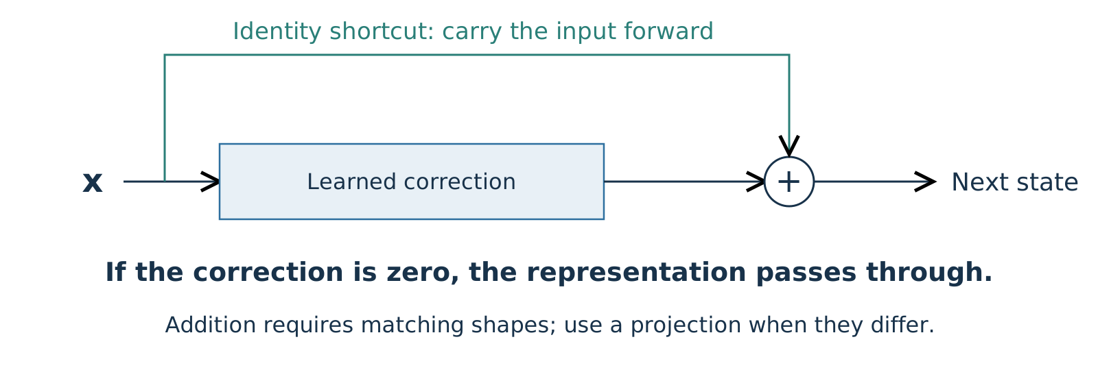
A residual block learns a change to the representation

\[\boldsymbol{x}_{\mathrm{next}}=\boldsymbol{x}+f(\boldsymbol{x})\]

About three minutes. Compare x_next=f(x) with x_next=x+f(x): learn a refinement while carrying the representation forward. The learned branch can contain several layers. Its output must match the input shape for addition. If channels or spatial size change, a learned projection replaces the identity shortcut. This diagram is the pure additive operation. Canonical ResNet-18 adds a ReLU after the sum, shown later, so zero branch output gives ReLU(x) there; it is identity on nonnegative block inputs, not arbitrary real inputs. [Sources] source:he-resnet-2016; source:torchvision-resnet-0-22.

Even a linear residual block starts from a different reference point

Replace the representation

\[\boldsymbol{x}_{\mathrm{next}}=W\boldsymbol{x}\]

Preserve the input: learn \(W=I\).

Near \(W=0\), the output is near zero.

Update the representation

\[\boldsymbol{x}_{\mathrm{next}}=(I+W)\boldsymbol{x}\]

Preserve the input: learn \(W=0\).

Near \(W=0\), the update is small.

Stacking linear residual blocks still gives a linear map. The change is how we parameterize learning, not the linear model’s expressivity.

About three minutes. W is square here; bias omitted. The same space of unconstrained linear maps can be expressed by W or I+W. A zero correction is an easy representation of identity, which motivates the residual parameterization for deeper nonlinear networks. Do not claim all training starts at exactly zero or that setting all parameters to zero is a good initialization. Keep random symmetry breaking and optimization separate. [Sources] source:he-resnet-2016.

The shortcut supplies a direct gradient contribution

For the additive block \(\boldsymbol{y}=\boldsymbol{x}+f(\boldsymbol{x})\):

\[\frac{\partial\boldsymbol{y}}{\partial\boldsymbol{x}} =I+\frac{\partial f(\boldsymbol{x})}{\partial\boldsymbol{x}}.\]

\[\frac{\partial L}{\partial\boldsymbol{x}} =\frac{\partial L}{\partial\boldsymbol{y}} +\left(\frac{\partial f(\boldsymbol{x})}{\partial\boldsymbol{x}}\right)^{\!T}\frac{\partial L}{\partial\boldsymbol{y}}.\]

The gradient has a path that does not multiply through the learned branch.

This helps explain deep residual networks; it does not guarantee stable gradients or better generalization.

About three minutes. Jacobian rows correspond to output entries, columns to input entries; gradients are column vectors. The first term follows the identity shortcut; the second follows the correction branch. Contributions can still cancel or grow, and many blocks still compose. The displayed formula is before any post-add activation. Canonical ResNet-18’s final ReLU contributes its own local derivative. Never equate residual connections with eliminating every vanishing/exploding-gradient problem. [Sources] source:he-resnet-2016.

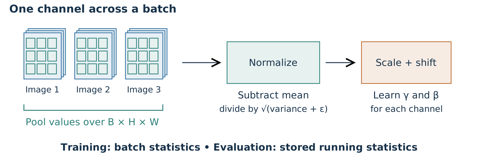
Batch normalization uses one set of statistics per channel

\[y_{bchw}=\gamma_c\frac{x_{bchw}-\mu_c}{\sqrt{v_c+\epsilon}}+\beta_c\]

About four minutes. For BatchNorm2d on B×C×H×W, compute each channel’s training mean and variance over B,H,W. Gamma and beta are trainable; mu and v are statistics, not gradient-trained parameters. Epsilon avoids division by zero. Standard PyTorch BatchNorm2d tracks running estimates and uses them in eval mode; this statement assumes track_running_stats=True. eval controls behavior, no_grad controls graph recording. Normalization is not an activation or input preprocessing; learned scale/offset can restore useful scales. Present conditioning/stability intuition without claiming an exclusive causal explanation or guaranteed training improvement. [Sources] source:pytorch-batchnorm2d-2-7.

Normalization layers differ in which values share statistics

Layer	Values grouped for each normalization
BatchNorm	One channel across examples and spatial positions
InstanceNorm	One channel’s spatial positions within one example
GroupNorm	A group of channels and spatial positions within one example
LayerNorm	Chosen trailing feature dimensions within one example

ResNet-18 uses BatchNorm. The U-Net example uses InstanceNorm.

The other three need no cross-example statistics. LayerNorm will return when we discuss transformers.

About two minutes; this is a pointer, not four separate derivations. For images the axes depend on tensor layout and configured normalized_shape. In transformers LayerNorm commonly normalizes the feature dimension independently per token. GroupNorm depends on the chosen number of groups. InstanceNorm by default uses per-input statistics in both training and evaluation; its affine parameters and tracking can be configured. Small batch behavior motivates alternatives, but no method is universally best. [Sources] source:pytorch-normalization-2-7; source:pytorch-instancenorm2d-2-7; source:pytorch-batchnorm2d-2-7; source:monai-basicunet-1-5-1.