Image Classification with ResNet (continued)

ECE 57000 — October 23, 2026

David I. Inouye

Architectural choices need evidence and a matching output

• CNN locality and sharing helped under our measured recipe, but did not guarantee shift robustness.
• Residual blocks add learned updates and a direct gradient path; normalization groups selected values.
• BatchNorm uses current-batch statistics during training and stored running statistics in default evaluation mode.

Today: finish ResNet-18 and U-Net, then define the prediction task for sequence models.

About two minutes. Recap October 21 and clarify the training/evaluation distinction: the live explanation used “inference” loosely while describing batch-statistic computation. The stored-statistic statement assumes PyTorch’s default track_running_stats=True. Learned gamma/beta differ from computed statistics; output standard deviation is approximately absolute gamma, not signed gamma, and epsilon matters. Residual direct paths do not guarantee nonvanishing total gradients. Repeat the final normalization comparison, then read pooling and the full classifier before changing the output task. [Sources] source:pytorch-batchnorm2d-2-7.

Normalization layers differ in which values share statistics

Layer	Values grouped for each normalization
BatchNorm	One channel across examples and spatial positions
InstanceNorm	One channel’s spatial positions within one example
GroupNorm	A group of channels and spatial positions within one example
LayerNorm	Chosen trailing feature dimensions within one example

ResNet-18 uses BatchNorm. The U-Net example uses InstanceNorm.

The other three need no cross-example statistics. LayerNorm will return when we discuss transformers.

About two minutes; this is a pointer, not four separate derivations. For images the axes depend on tensor layout and configured normalized_shape. In transformers LayerNorm commonly normalizes the feature dimension independently per token. GroupNorm depends on the chosen number of groups. InstanceNorm by default uses per-input statistics in both training and evaluation; its affine parameters and tracking can be configured. Small batch behavior motivates alternatives, but no method is universally best. [Sources] source:pytorch-normalization-2-7; source:pytorch-instancenorm2d-2-7; source:pytorch-batchnorm2d-2-7; source:monai-basicunet-1-5-1.

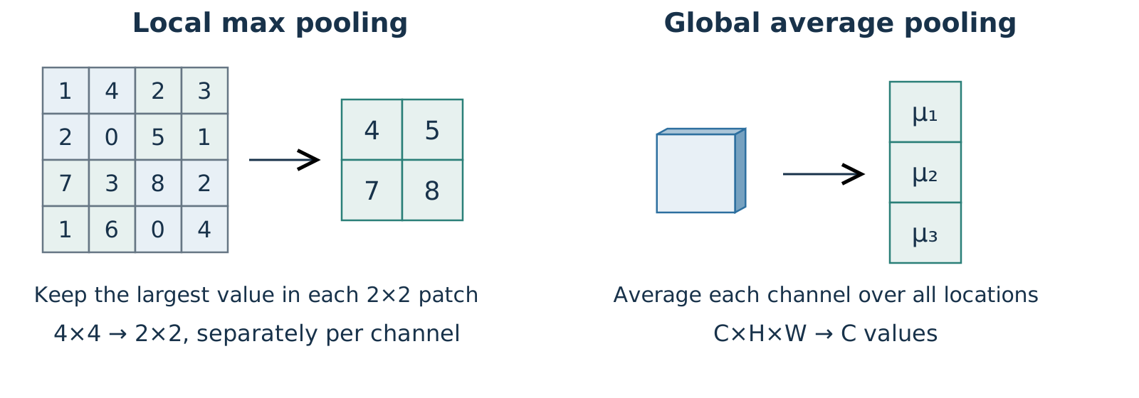
Pooling either reduces a map or summarizes each channel

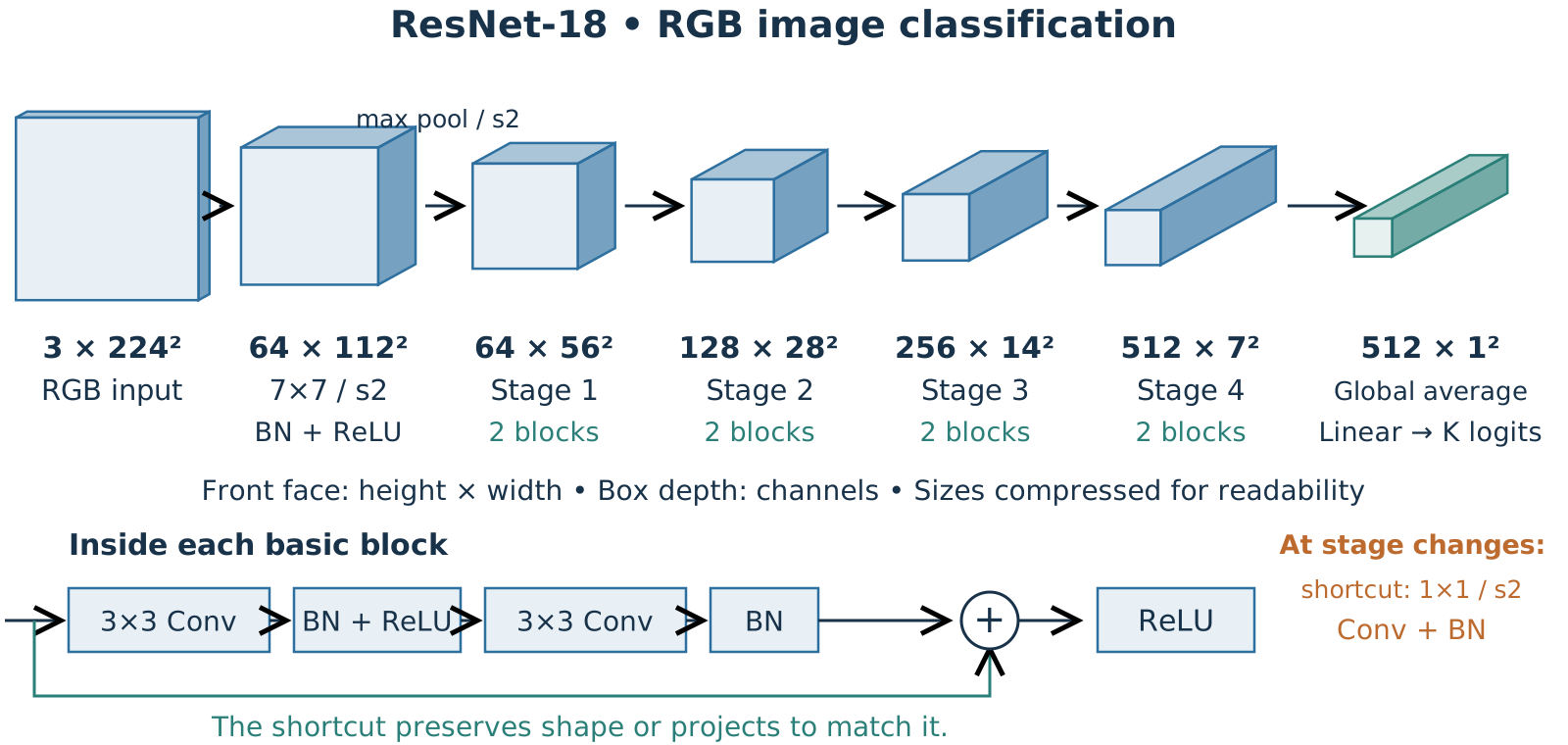
ResNet uses both: local pooling near the input; global averaging before the classification head.

About three minutes. Local illustration uses 2×2 nonoverlapping windows; ResNet’s stem instead uses a 3×3 max pool with stride 2 and padding 1. Pooling operates separately on channels and has no learned kernel. Global average pooling produces one value per channel; unlike flattening, it discards explicit spatial positions at this final step. Boundary effects and strides mean the whole network is not guaranteed exactly translation invariant. [Sources] source:torchvision-resnet-0-22.

ResNet-18 uses smaller spatial maps and more channels

Original illustration of torchvision ResNet-18; dimensions omit the batch axis.

About four minutes. Read the diagram left to right. The stem 7×7 stride-2 padding-3 Conv gives 112×112, then BN/ReLU and 3×3 stride-2 padding-1 max pool gives 56×56. Stage counts are [2,2,2,2] basic blocks. Stage 2/3/4 begin with stride-2 first convolution and a matching 1×1 stride-2 projection plus BN on the shortcut. The second convolution is stride 1. BN follows both branch convolutions; ReLU follows the first BN and the addition. Count 1 stem + 8×2 branch convolutions + 1 linear head = 18; shortcut projections are not counted in the naming convention. Global average pooling gives 512 features; ImageNet’s canonical head has K=1000 outputs, but a task can choose K. No network performance is implied. [Sources] source:torchvision-resnet-0-22; source:he-resnet-2016.

A prediction should not depend on unrelated batch companions

A trained BatchNorm classifier gives different scores for one image when its batch companions change.

What should you check first?

A. Whether model.eval() was called

B. Whether optimizer.zero_grad() was called

C. Whether the model needs more filters

A. Default BatchNorm uses stored running statistics in evaluation mode; training mode uses the current batch.

About three minutes including voting. Diagnose a deployment symptom using the normalization mechanism rather than assuming the architecture lacks capacity. Assume default PyTorch BatchNorm with track_running_stats=True and fixed weights; eval() also changes dropout behavior if present. zero_grad clears parameter gradients, not forward-pass statistics. More filters do not fix an accidental training/evaluation mode mismatch. Evaluation mode is distinct from no_grad/inference_mode. [Sources] source:pytorch-batchnorm2d-2-7.

Image Segmentation with U-Net

Segmentation needs a prediction at every image location

Arc 5: CNN fundamentals → evidence → ResNet classification → U-Net segmentation.

Task → Upsampling → Architecture

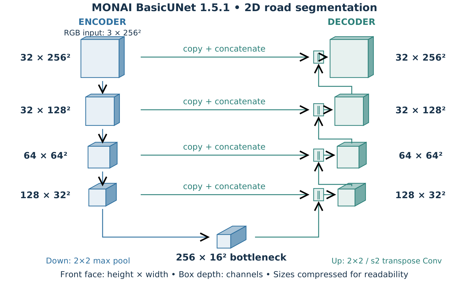
A classifier summarizes an image. A segmentation model must retain where each class occurs.

30-second transition. Introduce the changed output task before the new operation. We are predicting semantic classes, not identifying individual object instances. [Sources] source:ronneberger-unet-2015.

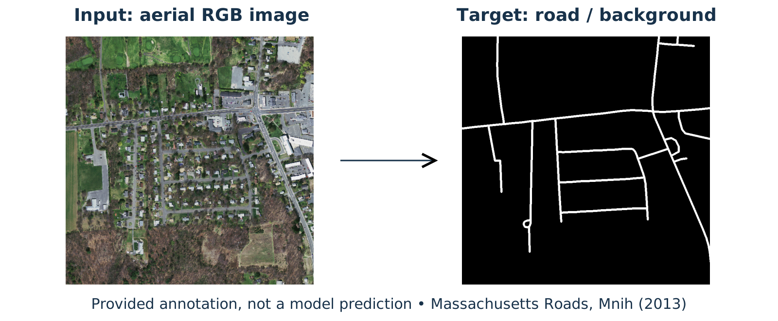
A road map needs a label at every pixel

Mnih, Massachusetts Roads (2013), validation tile 10228690_15; aligned crop.

About two minutes. A map-building system needs road locations, not just a road-present label. Input and provided annotation are cropped identically from (350,350) to (1150,1150) of a 1500×1500 tile. This illustrates supervision; the right image is neither a model prediction nor a performance evaluation. Masks are rasterized map targets and may not match every visible road edge; do not claim they are perfectly traced boundaries. Selecting this example does not define how to train or evaluate a model. [Sources] source:mnih-massachusetts-roads-2013; source:mass-roads-10228690-15-sat; source:mass-roads-10228690-15-map.

The input can stay the same while the output becomes spatial

	Image classification	Semantic segmentation
RGB input	\([B,3,H,W]\)	\([B,3,H,W]\)
Model logits	\([B,K]\)	\([B,K,H,W]\)
Integer targets	\([B]\)	\([B,H,W]\)

For roads: two logits per pixel, road or background.

Reuse cross-entropy, averaged over labeled pixels. Keep the spatial grid instead of globally pooling it away.

About two minutes. Brackets here denote tensor shapes, not matrix entries. Input need not acquire a new modality or channel; task labels and model output change. K is semantic class count, not number of instances. The two-logit binary setup reuses prior multiclass cross-entropy; a single-logit sigmoid/BCE version is an alternative outside this slide. Feed raw logits, not softmax probabilities, to PyTorch cross_entropy. Target ignore indices/missing labels require masking if present. Fashion-MNIST image categories are not segmentation masks. [Sources] source:ronneberger-unet-2015; source:monai-basicunet-1-5-1.

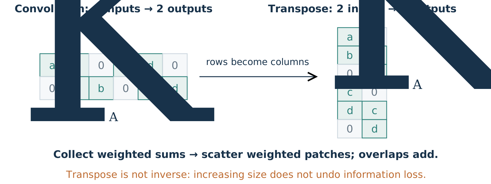
Transposed convolution uses the transpose of the linear operator

\[\boldsymbol{y}=A_K\boldsymbol{x}\qquad\longrightarrow\qquad\boldsymbol{u}=A_K^{\mathsf T}\boldsymbol{z}\]

About three minutes. Reuse the explicit 2×6 sparse operator from the recap and row-major vectorization. Each element of z scatters a weighted kernel patch back to the input lattice; overlaps add. This is the transpose of the input-to-output matrix for fixed kernel weights and compatible shape/boundary choices, not just transposing the small kernel image. Bias is omitted. The transpose is also the input-gradient operator. A decoder generally learns its own weights; it need not reuse an encoder’s kernel values. Reversing spaces does not make it an inverse or recover information removed by downsampling. [Sources] source:pytorch-convtranspose2d-2-7.

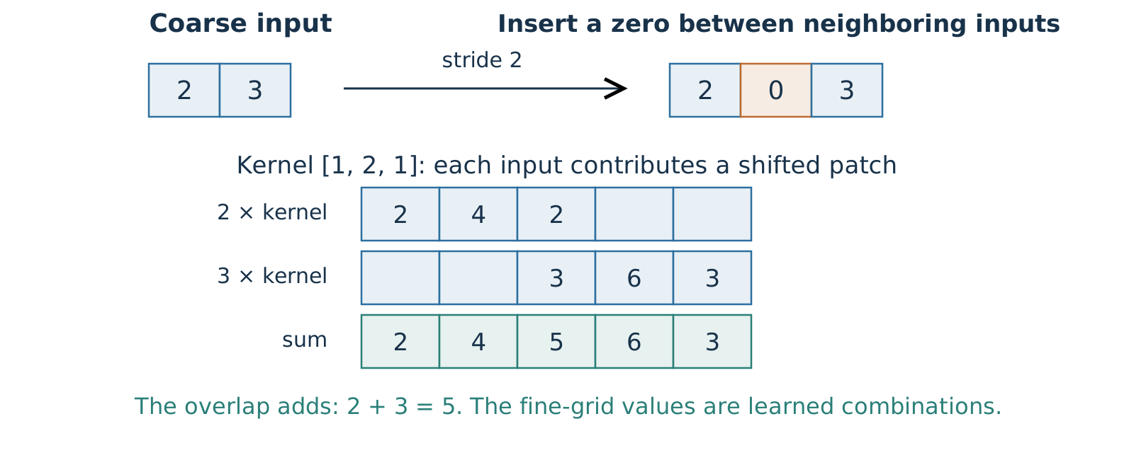
Fractional-stride intuition explains learned spatial expansion

In 2D, ConvTranspose2d(16, 8, 2, stride=2) maps \([B,16,16,16]\) to \([B,8,32,32]\).

About four minutes. The 1D example uses kernel [1,2,1], stride 2, padding 0: input [2,3] yields [2,4,5,6,3]. An equivalent implementation inserts one zero between inputs and applies a full filter, with appropriate boundaries and kernel orientation; the symmetric kernel deliberately avoids a distracting flip in this visual. For nonsymmetric PyTorch cross-correlation kernels the equivalent ordinary convolution requires the corresponding flip. Fractional stride describes the finer-grid interpretation, not a fractional stride argument in the API. The 2D doubling example uses kernel 2/stride 2/padding 0, so has no overlapping windows; it is separate from the overlapping 1D example. Learned expansion does not create observed evidence. Transposed convolution with stride 1 need not upsample. Interpolation followed by convolution is a common alternative; uneven overlap can matter for artifacts, beyond today’s scope. [Sources] source:pytorch-convtranspose2d-2-7.

U-Net combines coarse context with fine-resolution features

Original illustration of MONAI BasicUNet 1.5.1, 2D configuration; shapes are channels × spatial size.

About four minutes. Use spatial_dims=2, in_channels=3, out_channels=2, features=(32,32,64,128,256,32), upsample=‘deconv’, default instance normalization with affine=True and LeakyReLU slope .1. The image passes through the first two-convolution stage, then four max-pool/two-convolution stages. The decoder upsamples with 2×2 stride-2 transposed convolution, concatenates the matching encoder map, and applies two more Conv–InstanceNorm–LeakyReLU operations. Padding 1 preserves each stage’s spatial shape; 256 is divisible by 16. Default MONAI uses per-instance spatial statistics and learned scale/offset; do not label these blocks BatchNorm/ReLU. This is a contemporary maintained implementation of the U-Net family, not a claim of a universally best architecture. The original U-Net used valid convolutions with cropping; this padded version is easier to read. The input and output heads appear on the next slide. [Sources] source:monai-basicunet-1-5-1; source:ronneberger-unet-2015.

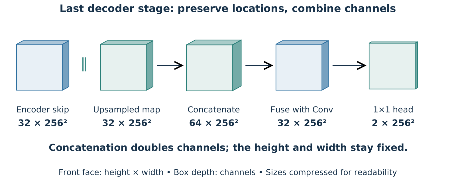
The U-Net head keeps one score vector at every pixel

About three minutes. This is the second and final complete-architecture explanation slide. In MONAI’s final UpCat, halves=False: the previous 32 channels remain 32 after upsampling, concatenate with the initial 32-channel skip, then TwoConv maps 64→32→32. A 1×1 convolution gives two logits per location. An argmax gives the predicted mask; per-pixel cross-entropy trains raw logits. At earlier upsampling stages channels halve before concatenation. Concatenation retains both feature sets, followed by learned fusion; it is different from adding an update to the same representation. Contrast the ResNet global-average-pooling + linear head with this spatial output. No residual blocks are required in this BasicUNet. [Sources] source:monai-basicunet-1-5-1.

The task determines what the architecture must preserve

• Classification: aggregate spatial features into an image-level decision.
• Segmentation: combine broad context with location-specific detail.
• Both: architectural choices need evidence on the intended data and task.

We can now read complete architectures from familiar operations. Knowing the pieces does not show that a model solves the application.

About two minutes. Close the arc without introducing another benchmark. For segmentation, pixel accuracy alone can hide missed roads because background can dominate; appropriate error measures and a held-out split would be needed before claiming usefulness. Return to the earlier Compare–Stress–Decide discipline, which preceded these architectural examples. Residual updates recur in transformers; encoder–decoder feature reuse recurs in generation. [Sources] source:ronneberger-unet-2015.

Sequence Prediction and Representation

David I. Inouye

Dynamic Content · Last Updated: October 23, 2026

A completion assistant needs a task, examples and a way to use context

Arc 6: Sequence-model architectures

1. Define the task: what is given, and what should come next?
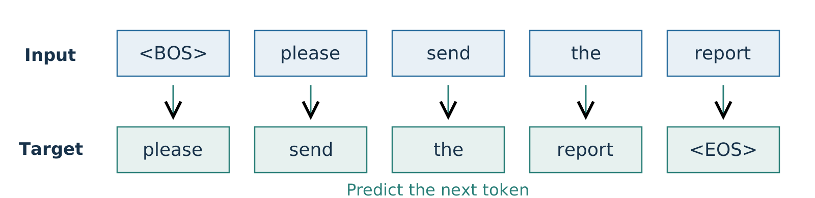
2. Build training examples: tokens, learned features and shifted targets.
3. Choose the context model: fixed window, recurrent state, then attention.

We will follow one email-completion example through each choice.

15-second map. Each step answers a question raised by the previous one. The CNN arc changed how models use spatial structure; this arc changes how models use ordered context. Return to these same three labels at the transition into recurrence. The later transformer/generation/systems sections continue the same email task.

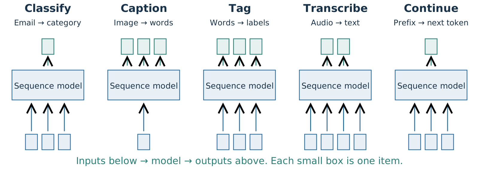
Sequence tasks differ in what goes in and what comes out

Our focus: next-token completion. Repeating it generates a continuation.

Original illustration informed by Karpathy’s sequence-task examples.

90 seconds. These show tasks, not a commitment to recurrent architecture. The middle block can use different sequence architectures. Classification may read the full message; next-token completion can only read its prefix. Tagging aligns an output to each input; transcription need not have equal input/output lengths. Image captioning uses one nonsequence input and a sequence output. For the completion pattern, feed the chosen next token back into the prefix to continue. This leads to choosing one concrete application. [Sources] source:karpathy-rnn-effectiveness-2015; source:d2l-rnn.

Email autocomplete suggests the next few words while you write

Typed prefix: “please send the”

Possible continuations: “report” · “slides” · “agenda”

• The writer supplies the message and accepts or ignores a suggestion.
• We predict the next token, then repeat to suggest a short continuation.
• Suggestions should fit the prefix and arrive quickly.

First: turn text into choices the model can predict.

Real application: Gmail Smart Compose (Chen et al., 2019). The email examples here are synthetic.

Two minutes. A concrete use case is completing routine work emails, not generating an entire email from a broad instruction. Smart Compose is evidence that completion is useful in a real product; these slides do not reproduce its model, dataset or measured performance. The toy example will use “please send the report” so every representation and recurrence can be followed by hand. Other listed suggestions illustrate ambiguity; the six-token arithmetic vocabulary below is intentionally smaller. No inbox access, personal messages or trained-model results are used. Later, a slow suggestion supplies the motivation for inference systems. [Sources] source:chen-smart-compose-2019.

Token IDs identify choices without ordering their meanings

Synthetic vocabulary for the worked examples:

Token	<BOS>	please	send	the	report	<EOS>
ID	0	1	2	3	4	5

please send the report becomes the ID sequence \((1,2,3,4)\).

• IDs select categories; subtracting two IDs does not measure similarity.
• A token can be a word, a word piece, punctuation, or a special marker.

Next: turn each ID into learned features.

About 90 seconds. BOS marks beginning and EOS marks end for our example; actual tokenizers may choose different conventions. The six-entry vocabulary is synthetic and intentionally tiny. A real word-level baseline fits its vocabulary only on training emails and reserves an unknown token. Subword vocabularies let common pieces compose many words; no tokenizer algorithm is needed now. Vocabulary size is v in equations and V in code-shaped tensors. [Sources] source:vaswani-attention-2017.

An embedding table learns features for each token

Synthetic table \(E\in\mathbb{R}^{6\times2}\):

Token	Feature 1	Feature 2
<BOS>	0	0
please	1	0
send	0	1
the	1	1
report	1	−1
<EOS>	−1	0

For token ID \(w_t=2\) (send):

\[\boldsymbol{e}_t=E^{\mathsf T}\boldsymbol{o}_2 =\begin{bmatrix}0\\1\end{bmatrix}\]

\(\boldsymbol{o}_2=[0,0,1,0,0,0]^{\mathsf T}\) selects row 2.

• Lookup selects the same learned row wherever a token occurs.
• Training updates that row through the prediction loss.

Next: specify the target that teaches these features.

About three minutes. All numbers are chosen for arithmetic, not learned from emails; the same table will be reused in the RNN trace. Zero-based token ID 2 indexes the third row. The one-hot vector is a conceptual selection device; implementations directly look up rows. E has v rows and d feature columns. Represent the selected row as a column vector e_t, hence E transpose times one-hot. Features need not have human-readable names; shared lookup alone gives identical features for repeated tokens, and the sequence model supplies context later. An embedding is neither a fixed semantic code nor a position encoding. [Sources] source:vaswani-attention-2017.

Each input position predicts the token immediately after it

\[\boldsymbol{p}_t=\operatorname{softmax}(\boldsymbol{z}_t), \qquad \ell_t=-\log p_{t,w_{t+1}}\]

Allowed context for \(\boldsymbol{z}_t\): tokens through \(w_t\) only.

Putting it together: one next-token prediction at each position.

About 2.5 minutes. z_t contains v vocabulary logits; p_t is the deterministic vector of predicted conditional probabilities. w_t is an observed integer token ID; p_{t,w_{t+1}} selects the probability assigned to the observed next ID. Reuse multiclass cross-entropy. With input positions 0 through T−1, targets use positions 1 through T. BOS lets the example predict its first ordinary token and EOS marks an ending. The target is available to compute loss, not to compute its own prediction. [Sources] source:d2l-rnn.