Sequence Prediction and Representation (continued)
ECE 57000 — October 26, 2026
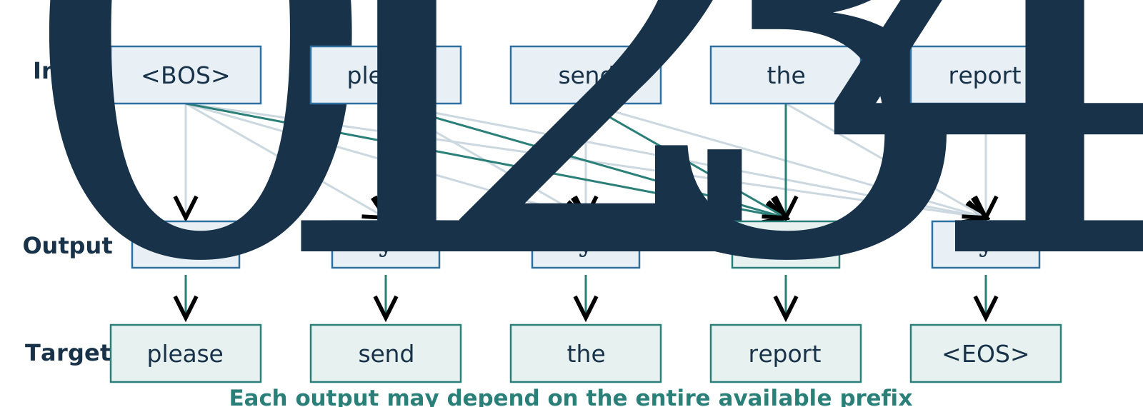
Next-token prediction connects text, learned features and targets
- Classification summarizes an image; segmentation preserves a prediction at every location.
- Token IDs select rows of a learned embedding table; ID differences do not measure meaning.
- Each prefix predicts the following token, using only the context available at that position.
Today: finish the training examples, then compare fixed windows, recurrent memory and attention.
The sequence model preserves positions while changing features
| Token IDs |
[B,L] |
Discrete input tokens |
| Input sequence \(X\) |
[B,L,d] |
Embedded rows \(\boldsymbol{x}_\ell\) |
| Hidden sequence \(H\) |
[B,L,h] |
Hidden-state rows \(\boldsymbol{h}_\ell\) |
| Output sequence \(Y\) |
[B,L,V] |
Logit rows \(\boldsymbol{y}_\ell\) |
| Target IDs |
[B,L] |
Next-token labels |
For one sequence: \(\boldsymbol{x}_\ell=X[\ell,:]\), \(\boldsymbol{h}_\ell=H[\ell,:]\), \(\boldsymbol{y}_\ell=Y[\ell,:]\) (rows).
Padding is absent data: exclude padded targets from the loss.
Test completion on held-out email threads
| Training threads |
Training prefixes and next-token targets |
| Validation threads |
Validation prefixes and next-token targets |
| Reserved test threads |
Final held-out prefixes and targets |
- Overlapping windows from one email share much of their text.
- Fit the vocabulary on training emails only; handle unseen tokens explicitly.
Now build a baseline: how much of the prefix should it read?
A fixed window turns continuation into familiar supervised prediction
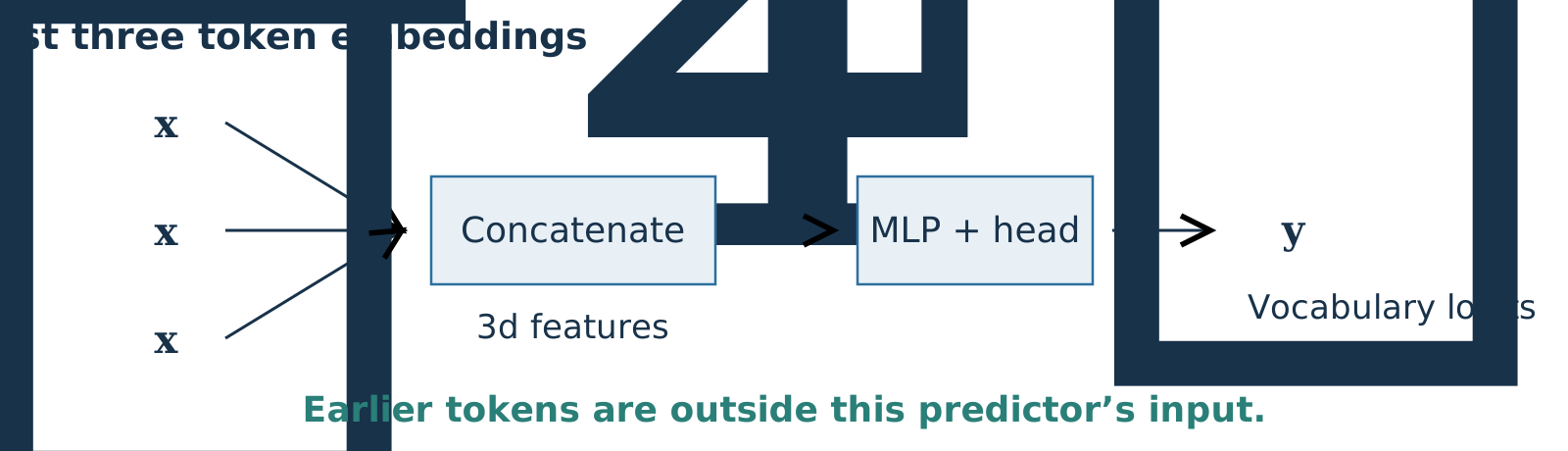
![The last three token embeddings are concatenated and passed through an MLP and a vocabulary head to produce next-token probabilities. Older tokens are outside this model's input.]()
\[\boldsymbol{y}_\ell=f_\theta\!\left(
[\boldsymbol{x}_{\ell-2}\;\boldsymbol{x}_{\ell-1}\;\boldsymbol{x}_\ell]\right)
\in\mathbb{R}^{v}\]
Its limitation: anything before the window is unavailable to the model.
Which change lets the model distinguish these contexts?
“Send the report today. Please attach the …”
“Send the slides today. Please attach the …”
Which change permits different predictions from a three-token model?
A. Add more hidden units
B. Include earlier tokens
C. Train on more emails
B. Identical input windows produce the same predicted distribution for fixed parameters.
Recurrent Neural Networks (RNN)
David I. Inouye
Dynamic Content · Last Updated: October 26, 2026
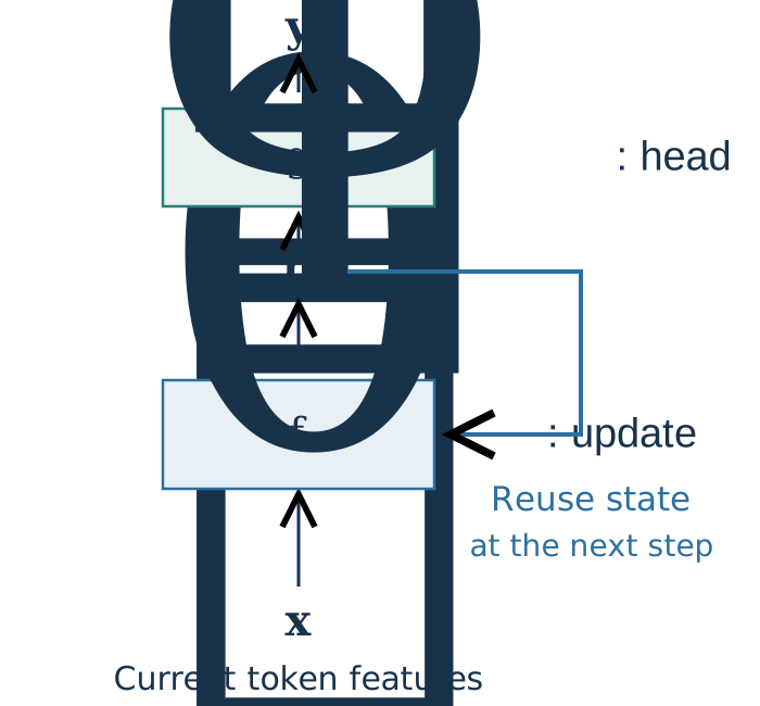
One transition combines the current token and the previous state
State update
\[\boldsymbol{h}_\ell=f_\theta(\boldsymbol{x}_\ell,\boldsymbol{h}_{\ell-1})\]
Vocabulary head
\[\boldsymbol{y}_\ell=g_\phi(\boldsymbol{h}_\ell)\]
The state changes with the prefix. The parameters \(\theta,\phi\) are shared.
Next: choose a concrete \(f_\theta\) and \(g_\phi\).
Familiar layers implement the recurrent update
\[\boldsymbol{h}_\ell=\operatorname{ReLU}\!\left(
\boldsymbol{x}_{\ell}W_x+\boldsymbol{h}_{\ell-1}W_h+\boldsymbol{b}\right)\]
\[\boldsymbol{y}_\ell=\boldsymbol{h}_{\ell}W_y+\boldsymbol{c},
\qquad\boldsymbol{p}_\ell=\operatorname{softmax}(\boldsymbol{y}_\ell)\]
| \(\boldsymbol{x}_\ell\in\mathbb{R}^{d}\) |
\(W_x\in\mathbb{R}^{d\times h}\) |
\(\boldsymbol{y}_\ell\in\mathbb{R}^{v}\) |
| \(\boldsymbol{h}_\ell\in\mathbb{R}^{h}\) |
\(W_h\in\mathbb{R}^{h\times h}\) |
\(W_y\in\mathbb{R}^{h\times v}\) |
\(f_\theta\): \(\theta=(W_x,W_h,\boldsymbol{b})\). \(g_\phi\): \(\phi=(W_y,\boldsymbol{c})\).
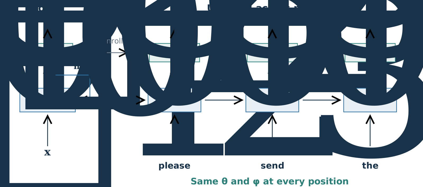
Unroll these shared functions to see the computation across the sequence.
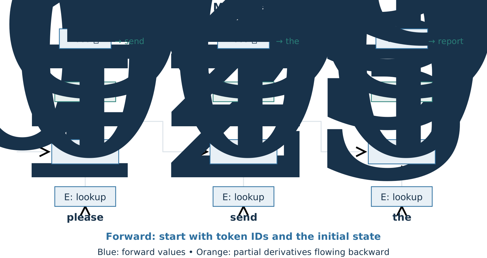
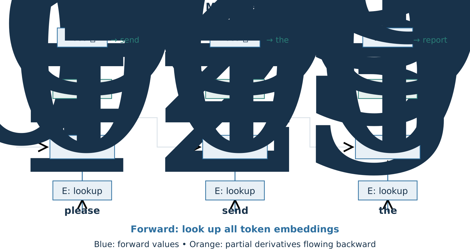
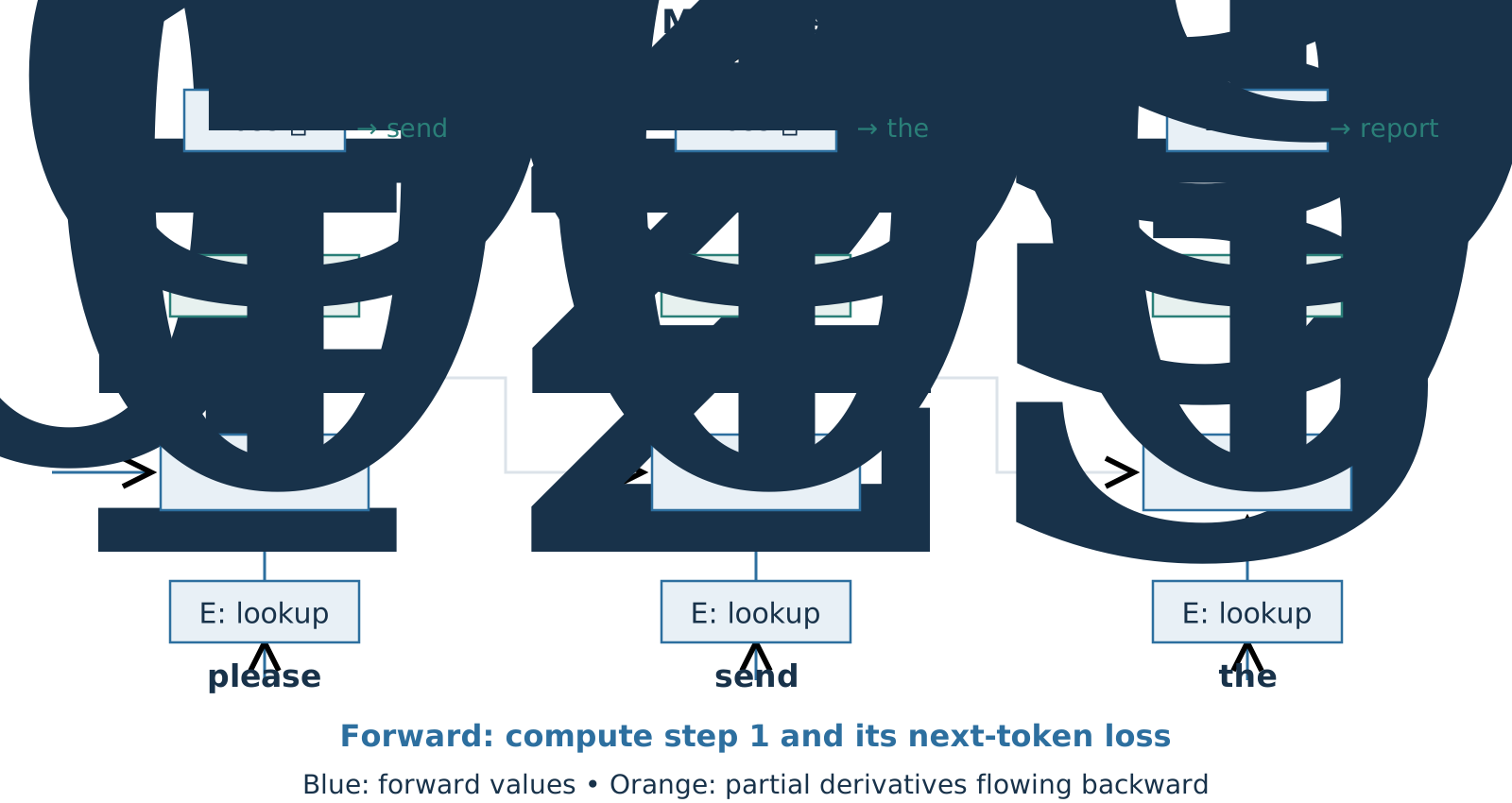
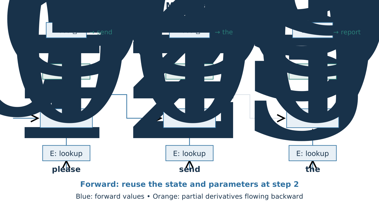
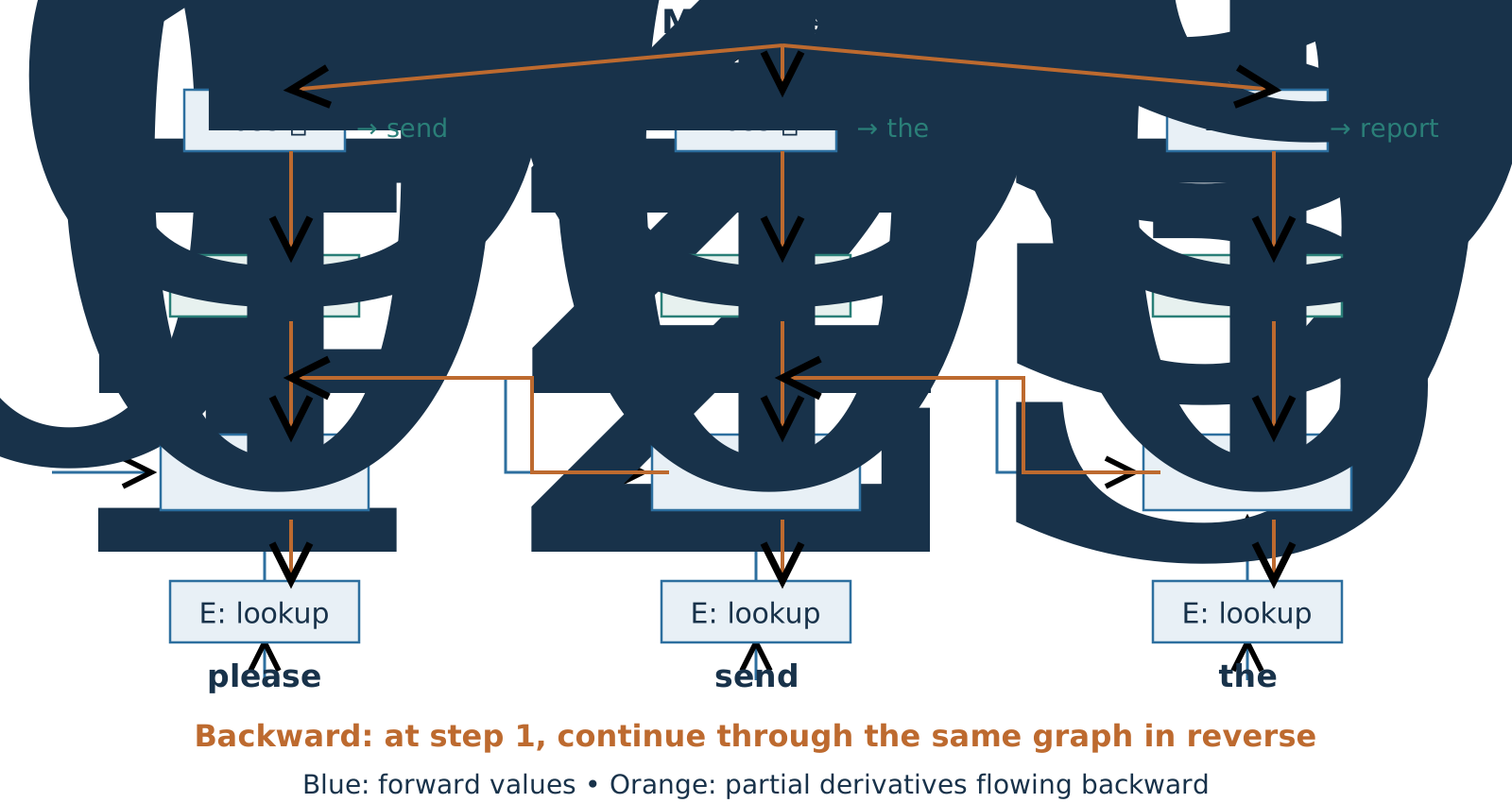
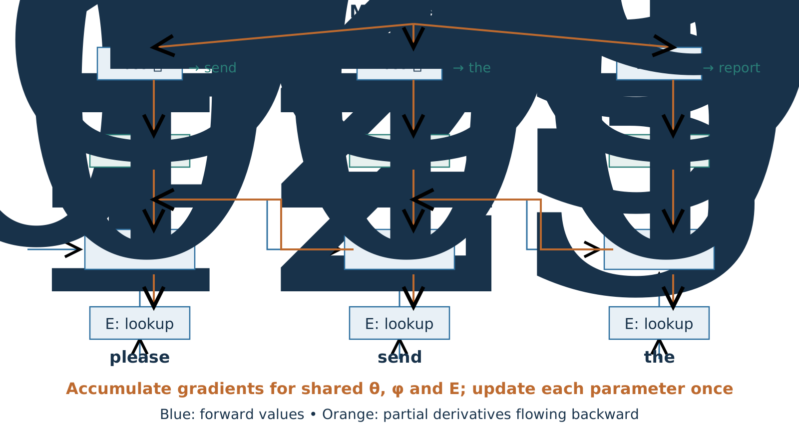
Unrolling repeats computation with shared parameters
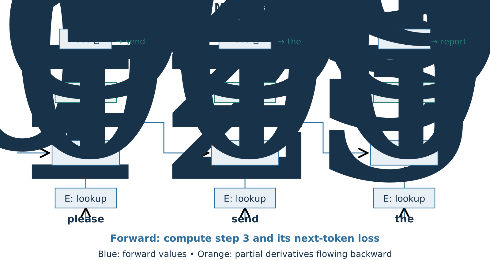
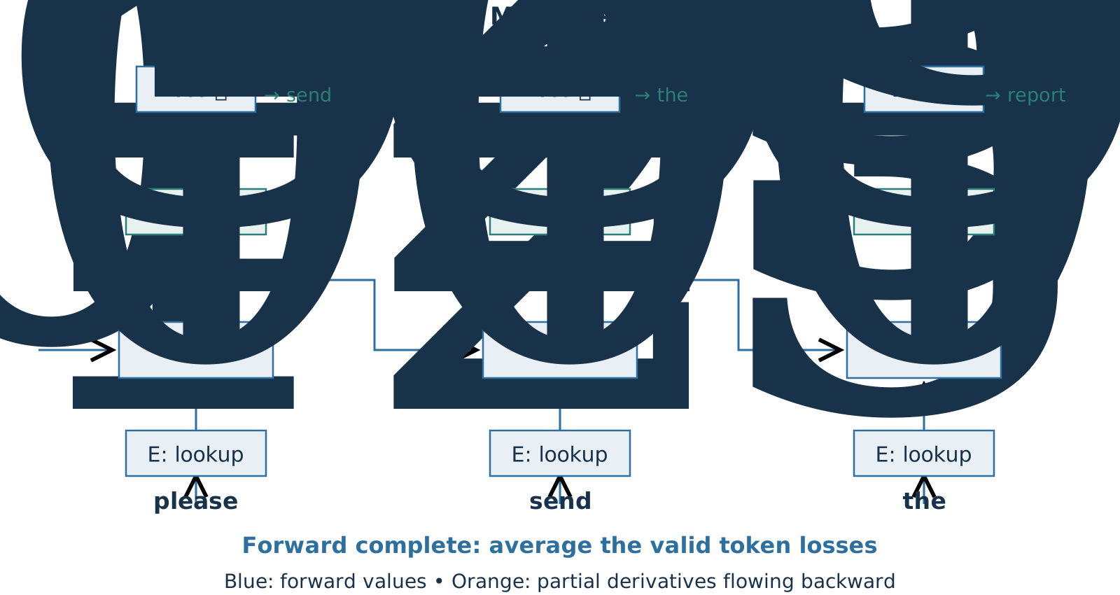
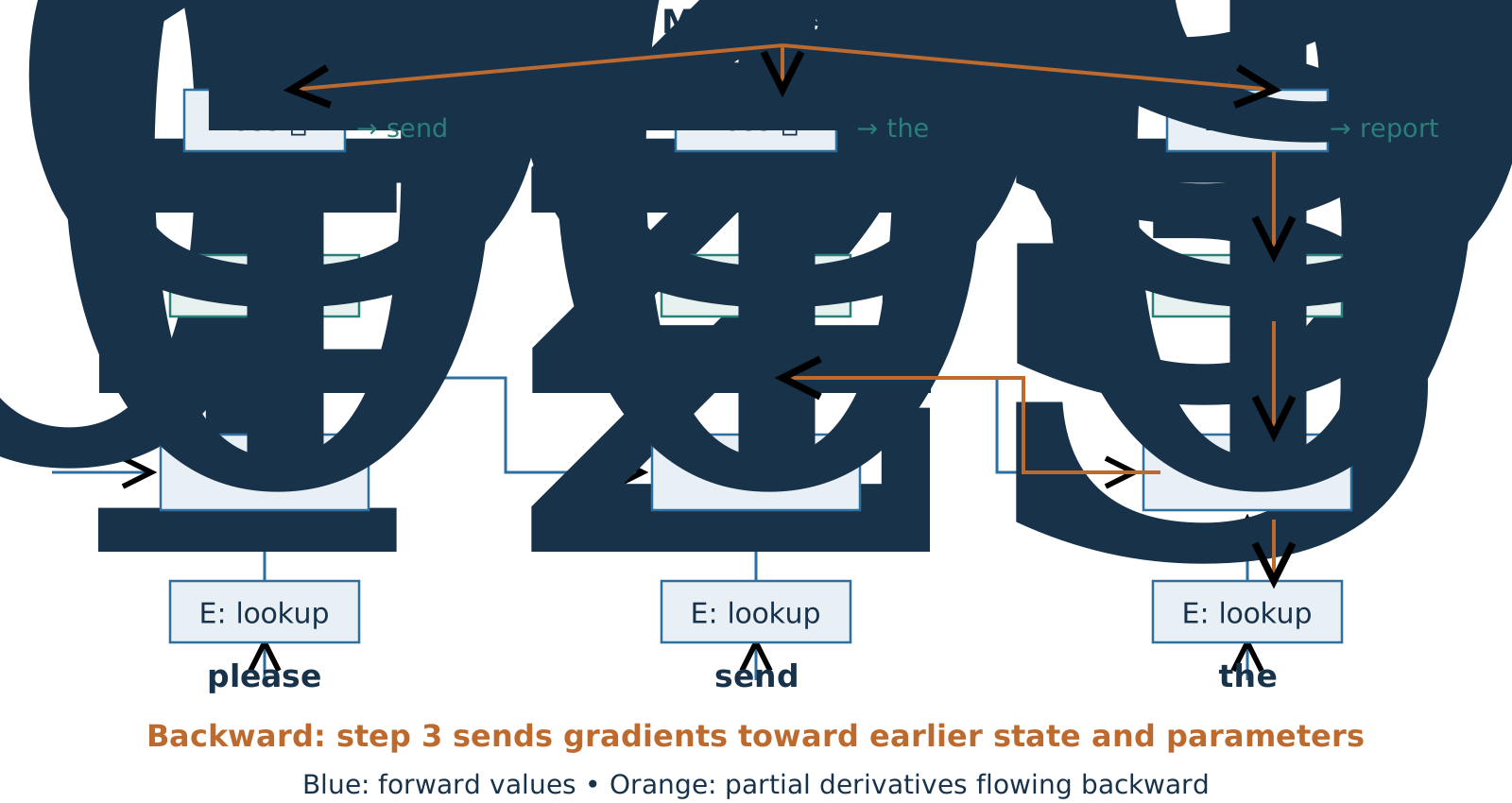
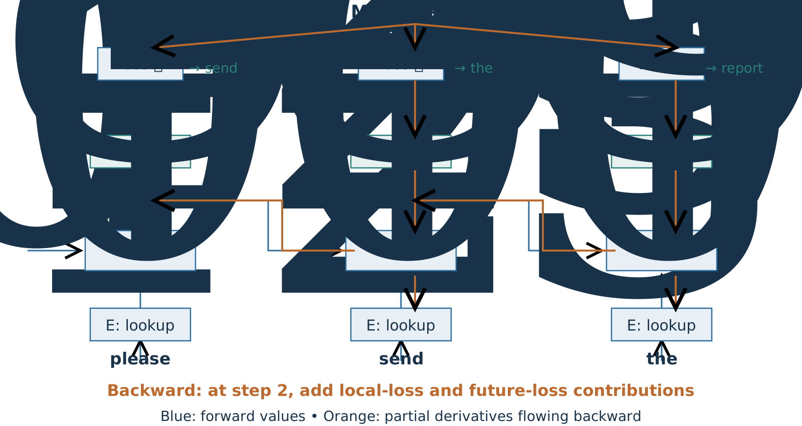
![The rolled recurrent cell is expanded into three vertical input-update-head columns for please, send, the. State passes from the initial zero vector through three steps. Each step has the same transition parameters and the same vocabulary-head parameters.]()
Three drawn cells are three uses of one learned transition.
Training assigns credit through the unrolled computation
Repeated derivatives can weaken or amplify distant credit
Scalar illustration: \(h_\ell=\operatorname{ReLU}(a h_{\ell-1}+x_\ell)\), with all relevant preactivations positive.
\[\frac{\partial h_\ell}{\partial h_{\ell-1}}=a,
\qquad
\frac{\partial h_\ell}{\partial h_{\ell-n}}=
\prod_{j=\ell-n+1}^{\ell}\frac{\partial h_j}{\partial h_{j-1}}=a^n\]
| \(a=0.5\) |
\(9.77\times10^{-4}\) |
\(9.54\times10^{-7}\) |
\(7.89\times10^{-31}\) |
| \(a=1.5\) |
\(57.7\) |
\(3.33\times10^3\) |
\(4.07\times10^{17}\) |
A longer path can make earlier information difficult to learn to preserve.
A longer message reuses the same learned transition
An RNN was trained on 20-token messages and receives a 30-token message.
What must grow to process the longer message?
A. The number of learned transition matrices
B. The number of recurrent computation steps
C. The width of each hidden state
B. More steps reuse the same parameters and state width.
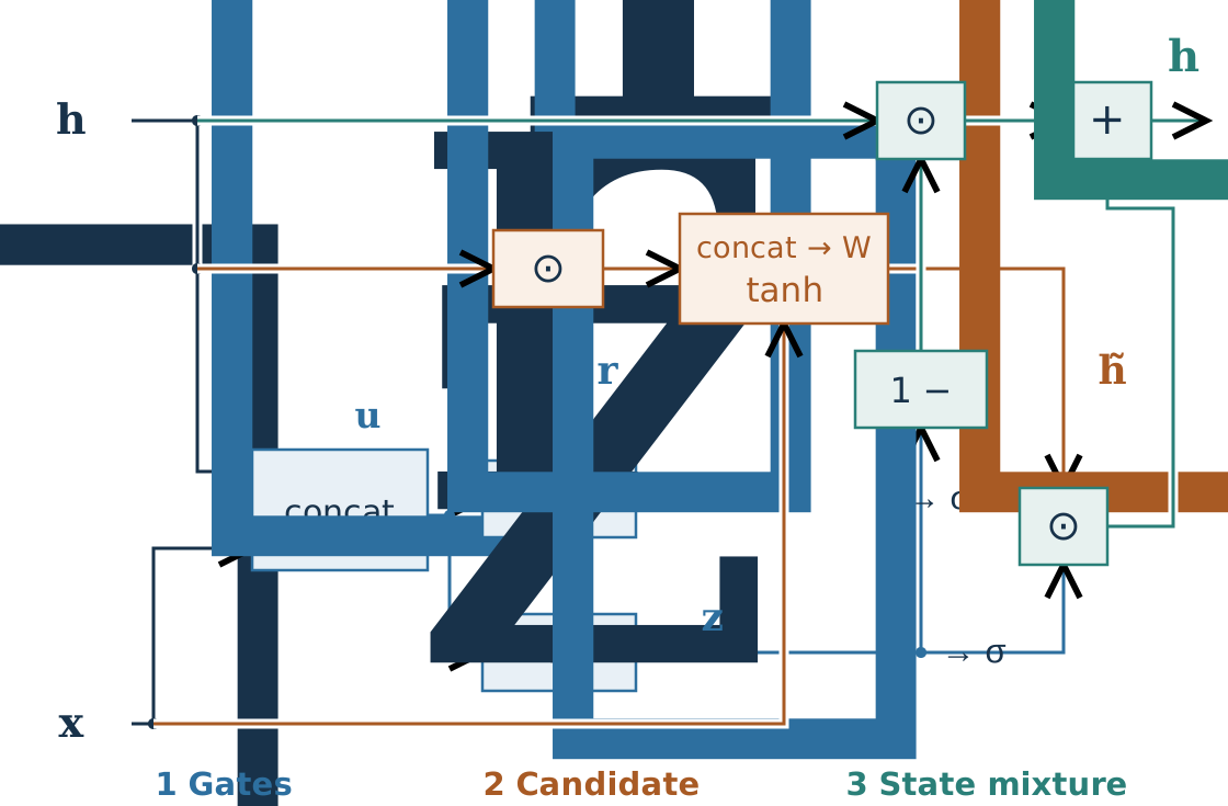
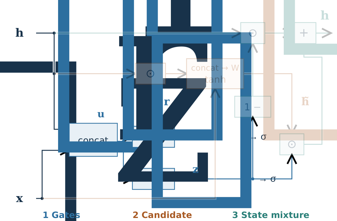
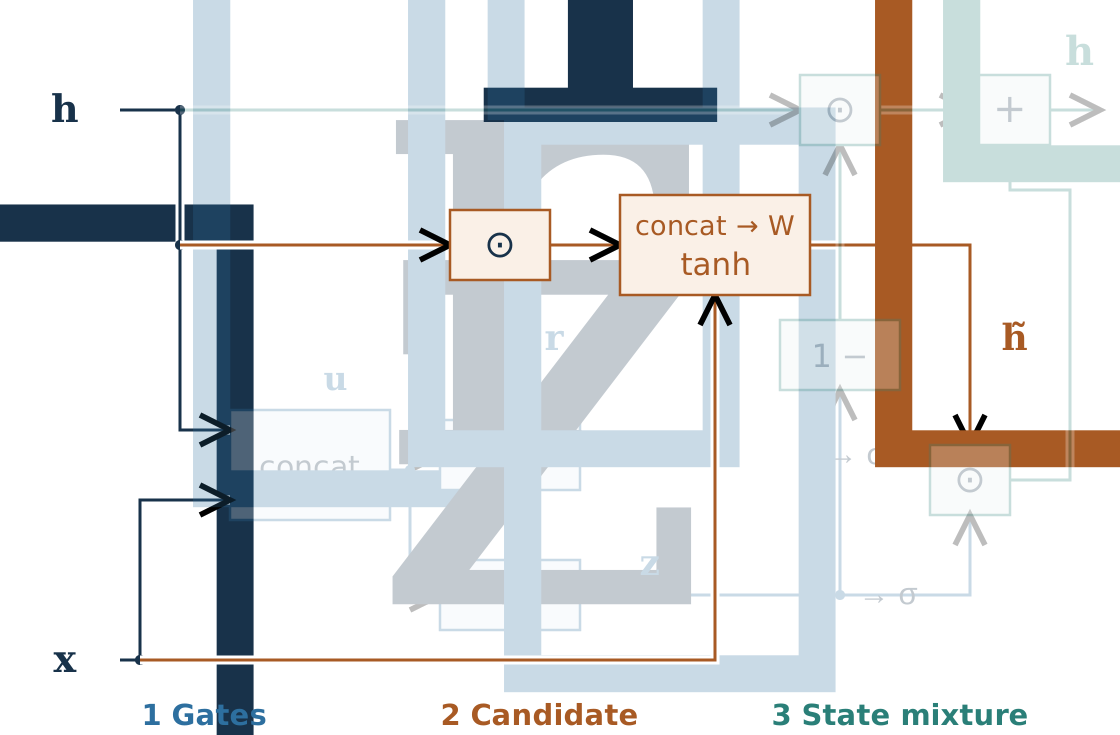
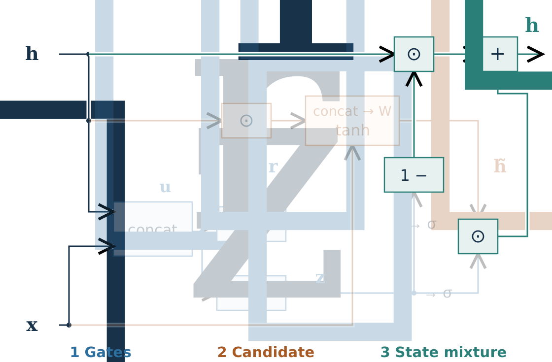
A GRU learns what to retain and what to replace
1 · Gates
\[\boldsymbol{u}_\ell=[\boldsymbol{h}_{\ell-1},\boldsymbol{x}_\ell]\] \[\color{#2D6F9F}{\boldsymbol{r}_\ell=\sigma(\boldsymbol{u}_\ell W_r),\quad
\boldsymbol{z}_\ell=\sigma(\boldsymbol{u}_\ell W_z)}\]
2 · Candidate
\[\color{#A85A24}{\widetilde{\boldsymbol{h}}_\ell=\tanh\!\left(
[\boldsymbol{r}_\ell\odot\boldsymbol{h}_{\ell-1},\boldsymbol{x}_\ell]W\right)}\]
3 · New recurrent state
\[\begin{aligned}\color{#2A7F78}{\boldsymbol{h}_\ell}
&\color{#2A7F78}{=(1-\boldsymbol{z}_\ell)\odot\boldsymbol{h}_{\ell-1}}\\
&\color{#2A7F78}{\quad+\boldsymbol{z}_\ell\odot\widetilde{\boldsymbol{h}}_\ell}
\end{aligned}\]
\(\boldsymbol{z}_\ell\approx\boldsymbol{0}\): retain old state. \(\boldsymbol{z}_\ell\approx\boldsymbol{1}\): use candidate.
LSTM: a common, more complex gated alternative with a separate cell state.
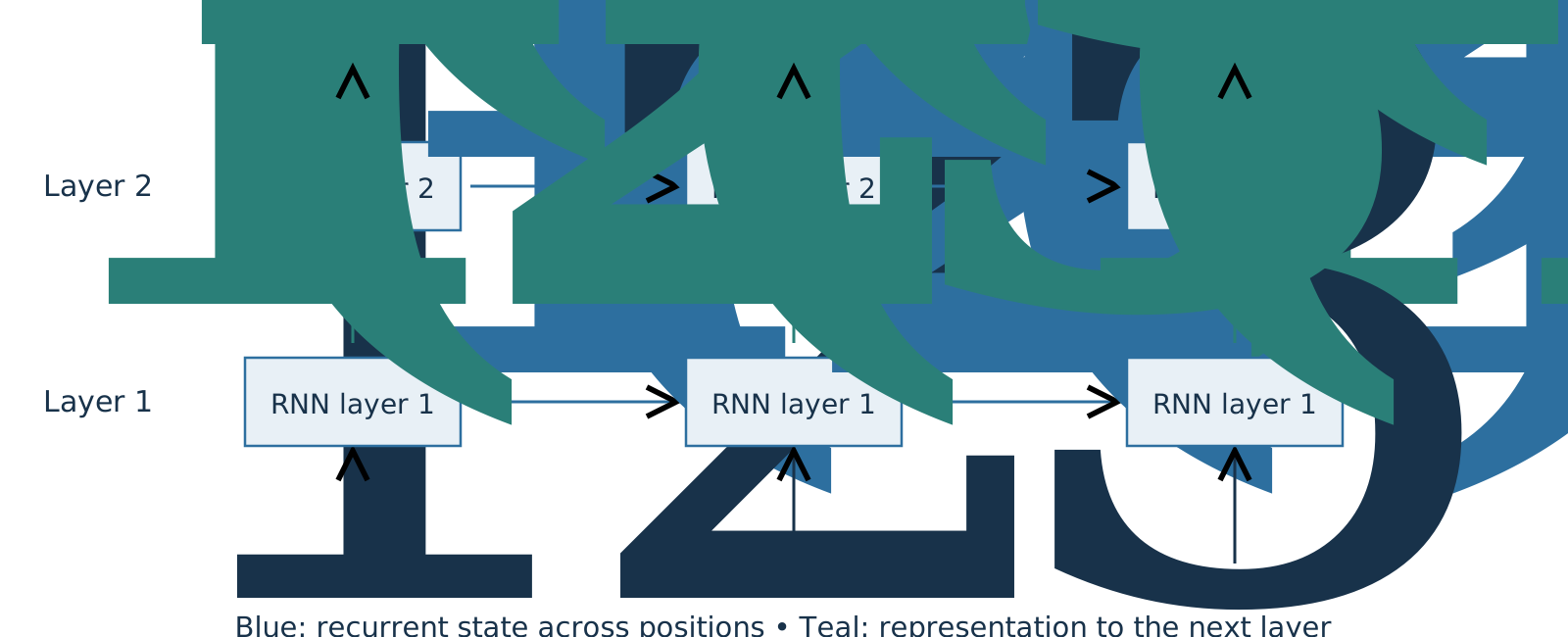
Deep RNNs stack recurrent layers
![Two recurrent layers across three positions: inputs feed layer one; z representations pass upward and h recurrent states pass horizontally, with explicit position subscripts and layer superscripts.]()
Horizontal: \(\boldsymbol{h}_\ell^{(k)}\), recurrent state. Vertical: \(\boldsymbol{z}_\ell^{(k)}\), layer representation.
For vanilla RNNs and GRUs, \(\boldsymbol{z}_\ell^{(k)}=\boldsymbol{h}_\ell^{(k)}\): same value, different role.
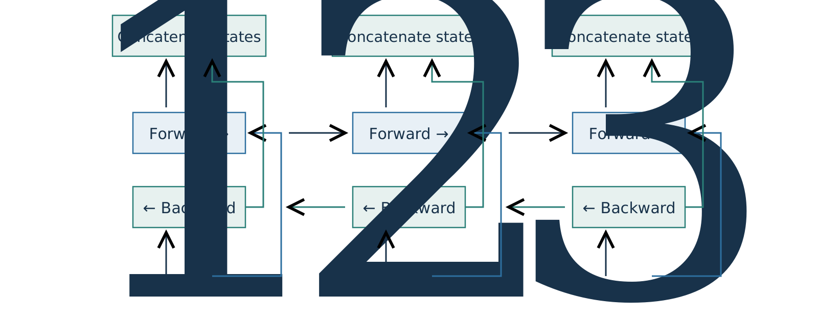
Bidirectional RNNs combine left and right context
![One RNN traverses the input left to right and another right to left. Their states at each position are concatenated into one representation.]()
Useful when the whole input is available, such as tagging a complete sentence.
Not valid for next-token prediction if the backward state can see the target.
A small RNN improves held-out email next-token prediction
Measured AESLC email-body experiment: 13,415 train / 1,769 validation / 1,604 test emails.
| Bigram: use only the previous token |
4.840 |
18.9% |
| One-layer RNN: use the prefix |
4.454 |
23.3% |
- At most 64 tokens/email; shared 4,000-token vocabulary; one training seed.
- 6.5% of test targets become
<UNK>; accuracy on known targets is 17.3% vs. 21.8%.
Synthetic prompt, measured predictions: please send the → attached, following, latest.
Next comparison: freeze these data, tokens and metrics; replace the RNN with attention.