Recurrent Models and Attention

ECE 57000 — October 28, 2026

David I. Inouye

Shared recurrent computation learns from every prediction loss

• Shift targets by one token; split whole emails before forming training examples.
• Reuse one transition across positions; BPTT accumulates gradients through every use.
• GRU gates mix retained state with candidate content; longer sequences still require more steps.

Today: finish the RNN limitations, then replace the state chain with attention.

About two minutes. October 26 covered fixed windows, recurrence, BPTT, gradient products, GRU, deep/bidirectional variants, PyTorch and a brief measured email result. A student asked about detaching hidden states: this omits gradient paths and does not remove forward sequential dependence. Gates and additive retention can help, but bounded states do not guarantee bounded full Jacobians or stable gradients. The displayed RNN result was a single-seed next-token comparison, not a product-quality claim; the bigram uses one previous token. Repeat the displayed but deferred limitations slide next. [Sources] source:d2l-bptt; source:olah-understanding-lstms-2015; source:aeslc-2019.

Recurrent memory creates information and training bottlenecks

Limitation	Why it matters
Fixed-width memory	Earlier information must survive repeated state updates; a final-state summary must represent the whole sequence.
Long gradient paths	Distant credit passes through many Jacobians, complicating optimization.
Sequential computation	State \(\boldsymbol{h}_\ell\) must wait for \(\boldsymbol{h}_{\ell-1}\), limiting training parallelism across positions.

Next: retain all position representations and combine them directly.

Three minutes. RNNs can retain all their outputs, but their contextual computation still routes through the recurrent chain; do not claim all RNNs discard all earlier states. A single-vector encoder is the especially clear compression case. Gates help memory but do not remove the sequential dependency. Parallel computation during training was a major motivation for replacing recurrence with self-attention in transformers; RNNs remain useful in some settings. Distinguish optimization through long paths from hardware throughput. Attention shortens paths and removes this within-layer chain, not every training difficulty. [Sources] source:d2l-bptt; source:vaswani-attention-2017, sections 1 and 4.

Attention and Position

David I. Inouye

Dynamic Content · Last Updated: October 26, 2026

Self-attention combines representations from the same sequence

Arc 6: Sequence-model architectures → Attention and position

1. Write the complete self-attention equation.
2. Unpack its input-dependent soft lookup.
3. Extend to cross-attention, then restrict access for our next-token task.

Position information comes next.

Thirty seconds. This is a pedagogical order, not a historical account: self-attention first, cross-attention as an extension. Begin with the full matrix equation, then connect it to the familiar weighted combination and dictionary analogy. [Sources] source:vaswani-attention-2017.

Self-attention is one input-dependent matrix operation

Input \(X\in\mathbb{R}^{L\times d}\): one row per position. Biases omitted.

Projection	Learned matrix	Result shape
\(Q=XW_Q\)	\(W_Q\in\mathbb{R}^{d\times d_k}\)	\(L\times d_k\)
\(K=XW_K\)	\(W_K\in\mathbb{R}^{d\times d_k}\)	\(L\times d_k\)
\(V=XW_V\)	\(W_V\in\mathbb{R}^{d\times d_v}\)	\(L\times d_v\)

\[A=\operatorname{softmax}_{\rm row}\!\left(\frac{QK^{\mathsf T}}{\sqrt{d_k}}\right) \in\mathbb{R}^{L\times L},\qquad Y=AV\in\mathbb{R}^{L\times d_v}\]

Attention matrix \(A\): input-dependent weights, one row per output position.

\[\operatorname{SA}(X)= \operatorname{softmax}_{\rm row}\!\left(\frac{(XW_Q)(XW_K)^{\mathsf T}}{\sqrt{d_k}}\right)(XW_V)\]

Three minutes. Present the complete scaled dot-product equation first, then unpack it over the following slides. W_Q and W_K are d by d_k, W_V is d by d_v; Q/K have L rows and V/Y have L rows and d_v columns. Show the dimension match: Q times K transpose is (L by d_k)(d_k by L), giving L by L. Row softmax preserves this shape. A times V is (L by L)(L by d_v), giving L by d_v. A has one query/output position per row and one key/input position per column; every row sums to one. The batch axis is omitted here; code uses A of shape [B,L,L]. The weight matrices are fixed learned parameters at inference; A is recomputed from the input. Row softmax normalizes over input/key positions for each output/query position. d_k is query/key feature width. There is no recurrent state chain in this formula. All input positions are available here; task-specific restrictions come later. X can hold embedded inputs or previous-layer representations. One head, no bias, dropout or output projection. Cross-attention is introduced only after self-attention. [Sources] source:vaswani-attention-2017, section 3.2.

Self-attention combines inputs directly, with input-dependent weights

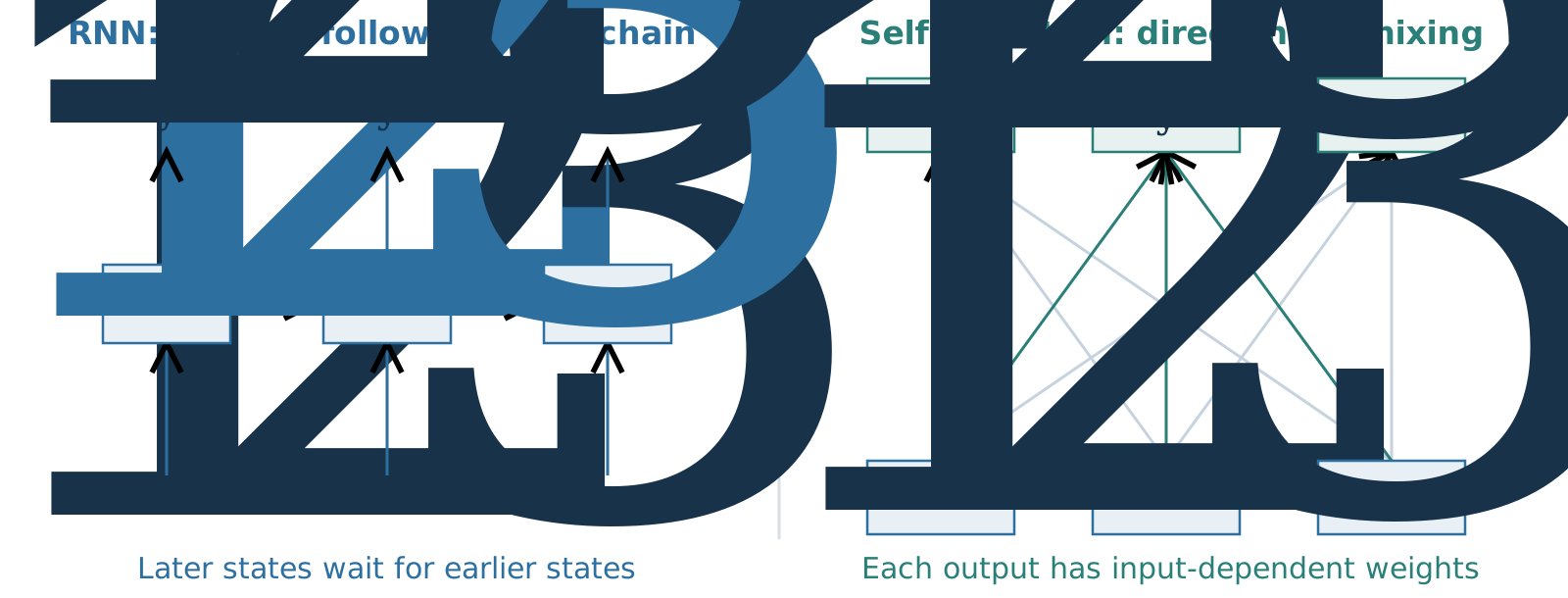
Each \(\boldsymbol{y}_\ell\) combines information from all rows of \(X\).

The learned projection matrices stay fixed; the combination weights are input-dependent.

2.5 minutes. Compare the RNN chain on the left with the direct dependencies on the right. Follow the highlighted middle attention output, then the others. The new states depend on the input states of this layer, not on each other’s newly computed outputs. This avoids a circular definition and explains why they can be computed together. We retain all input rows instead of forcing the whole history through a final recurrent summary. Outputs still have fixed feature width; memory cost grows with sequence length. [Sources] source:vaswani-attention-2017, sections 3.2 and 4.

Self-attention removes the sequential chain within a layer

RNN	Self-attention
\(\boldsymbol{h}_1\rightarrow\boldsymbol{h}_2\rightarrow\cdots\rightarrow\boldsymbol{h}_L\)	\(X\rightarrow\{\boldsymbol{y}_1,\ldots,\boldsymbol{y}_L\}\) together
Distant information travels through successive updates	Each output directly combines all input positions
Position \(\ell\) waits for the preceding state	Outputs share the same available input collection

Shorter paths for learning; parallel operations across positions during training.

Two minutes. A single dense self-attention layer connects arbitrary positions directly, avoiding the recurrent path’s length dependence. This aids access and gradient flow but does not guarantee easy optimization. Matrix operations expose training parallelism when all layer inputs are available. Layers still depend on earlier layers, and generating new autoregressive tokens remains sequential. Dense attention also has quadratic pairwise score cost; discuss that tradeoff later in systems. Early attention over RNN outputs helped the compression bottleneck; replacing recurrence with self-attention also removed the recurrent training chain. [Sources] source:vaswani-attention-2017, sections 1 and 4.

Attention builds an input-dependent weighted combination

For each input row, form a value: \(\boldsymbol{v}_j=f_v(\boldsymbol{x}_j)=\boldsymbol{x}_jW_V\).

\[\boldsymbol{y}_\ell=\sum_{j=1}^{L}a_{\ell j}\boldsymbol{v}_j, \qquad a_{\ell j}\geq0,\quad\sum_{j=1}^{L}a_{\ell j}=1\]

• The score for pair \((\ell,j)\) is a function of both inputs: \(s_{\ell j}=f_s(\boldsymbol{x}_\ell,\boldsymbol{x}_j)\).
• \(a_{\ell j}=\operatorname{softmax}_j(s_{\ell1},\ldots,s_{\ell L})\): normalize against all candidate inputs.

How do queries and keys turn these input pairs into useful weights?

Two minutes. Values and scores are learned functions of inputs; the model does not learn one fixed attention matrix. More precisely the pair score depends on x_ell and x_j, but its normalized weight depends on all keys through the denominator. Therefore do not write a_ell,j=f_a(x_ell,x_j) as if changing another input could not affect this weight. For scaled dot-product attention f_s=(x_ell W_Q)(x_j W_K)^T/sqrt(d_k). Each output is a convex combination for this one ordinary softmax head; the complete transformer is not a convex model. No future-token restriction yet. [Sources] source:vaswani-attention-2017.

Attention is a soft lookup in a key–value table

Dictionary lookup: an exact key selects one stored value.

Attention: a query scores every key, then blends the paired values.

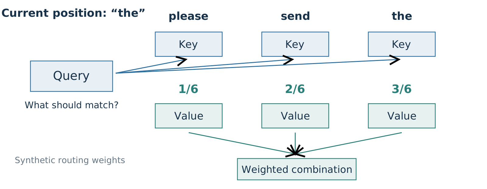
Query: features to match. Key: matching features. Value: features to combine.

Three minutes. These are three learned representations, not literal natural-language questions, database strings or dictionary definitions. Each source position supplies a paired key and value. The query-key match decides a weight, which multiplies the corresponding value. The displayed weights will be calculated on the next example; they are synthetic and carry no semantic or causal-explanation claim. [Sources] source:vaswani-attention-2017.

Softmax turns matching scores into relative combination weights

\[s_{\ell j}=\frac{\boldsymbol{q}_\ell\boldsymbol{k}_j^{\mathsf T}}{\sqrt{d_k}}, \qquad a_{\ell j}=\frac{\exp(s_{\ell j}-m_\ell)}{\sum_{k=1}^{L}\exp(s_{\ell k}-m_\ell)}, \qquad m_\ell=\max_{k} s_{\ell k}\]

• A larger dot product gives a larger weight relative to the other scores.
• Subtracting the row maximum preserves the weights and avoids large exponentials.

These weights are not probabilities that a token is true or important.

Next: calculate one complete weighted combination.

Three minutes. Reuse the earlier multiclass softmax computation but distinguish its role: here it normalizes source-position scores, not vocabulary logits. Queries and keys have the same width; values can have a different width. The next toy has key/query width one so the standard scale factor is one. The scale already appears in the full equation; explain its magnitude correction after the example. Attention weights alone do not show the causal influence of an input on a model’s final decision. [Sources] source:vaswani-attention-2017.

One weighted combination uses values, not token IDs

Synthetic one-feature query \(\boldsymbol{q}=[1]\); the query is at the.

Source token	Key	Score	Softmax weight	Value \(\boldsymbol{v}_j\)
please	\([0]\)	\(0\)	\(1/6\)	\([1,0]\)
send	\([\log2]\)	\(\log2\)	\(2/6\)	\([0,2]\)
the	\([\log3]\)	\(\log3\)	\(3/6\)	\([2,2]\)

\[\boldsymbol{y}=\tfrac16[1,0]+\tfrac26[0,2]+\tfrac36[2,2]=[7/6,5/3]\]

This is a context feature vector. A later vocabulary head predicts the next token.

Four minutes. Natural logs give unnormalized weights 1,2,3 and denominator 6. Calculate each output entry. These hand-chosen query/key/value vectors are a new synthetic operator example, not the earlier embedding rows or a trained projection of them. Key width is one and value width is two. The formula is checked by arc6_attention_diagrams.py. Keep logits and routing weights distinct. [Sources] source:vaswani-attention-2017.

Matrix multiplication computes all output states together

Stack token representations as rows of \(X\in\mathbb{R}^{L\times d}\).

\[S=QK^{\mathsf T}/\sqrt{d_k},\qquad A=\operatorname{softmax}_{\rm row}(S),\qquad Y=AV\]

Object	Shape	Meaning
\(Q,K\)	\(L\times d_k\)	Query/key features per token
\(QK^{\mathsf T}\)	\(L\times L\)	Query rows × key columns
\(A\)	\(L\times L\)	One normalized weight row per query
\(Y=AV\)	\(L\times d_v\)	Combined value features per token

One row of \(A\) gives the input-dependent weights for one output row of \(Y\).

3.5 minutes. L is the number of input positions; omit the batch axis in the displayed matrices. In code X is [B,L,d], Q and K are [B,L,d_k], V is [B,L,d_v], A is [B,L,L], and Y is [B,L,d_v]. Transpose only the last two axes of K. Values V have shape L by d_v. Multiply one row of A by V to recover the numeric example. All rows can be evaluated together when input representations are available; this does not yet explain autoregressive generation. Scaling preserves these shapes; the later mask will modify scores without changing shapes. The attention weights A are distinct from learned projection parameters. [Sources] source:vaswani-attention-2017.

Divide by \(\sqrt{d_k}\) to keep score fluctuations comparable

Assume independent query/key entries with mean \(0\) and variance \(1\).

\[z=\boldsymbol{q}\boldsymbol{k}^{\mathsf T}=\sum_{i=1}^{d_k}q_i k_i, \qquad \mathbb{E}[z]=0,\qquad \operatorname{Var}(z)=d_k\]

Positive and negative terms partly cancel. Variances add; standard deviations grow as \(\sqrt{d_k}\).

Dividing by \(\sqrt{d_k}\) keeps the score standard deviation at \(1\), for any width.

Example, \(d_k=20\): two keys with a score gap of \(\sqrt{20}\approx4.47\).

Scores	Softmax weights
\([0,\sqrt{20}]\)	\([1.1\%,98.9\%]\)
Divide by \(\sqrt{20}\): \([0,1]\)	\([26.9\%,73.1\%]\)

Avoid near-one-hot attention caused merely by width: saturated softmax has small gradients.

Three minutes. Original Transformer section 3.2.1 and footnote 4 supply this argument. Assume all entries of q and k are independent, zero-mean and unit-variance; standard normals are one example, but normality is unnecessary. Each product has mean zero and variance one because E[q_i^2 k_i^2]=1; independent products have additive variances. The root-mean-square score equals sqrt(d_k), although the signed expected score remains zero. This is like a random walk: signs partly cancel, but the spread grows. Dividing by sqrt(d_k) cancels the standard-deviation growth; dividing by d_k would shrink it as 1/sqrt(d_k). If terms were aligned or had nonzero means, a linear-in-width sum could occur, but that is not the paper’s model. The assumption concerns projected query/key features, not projection weights: unit-variance W entries alone do not give unit-variance Q/K, and actual feature correlations/scales can differ.

The displayed two-key scores are deliberately chosen, not a simulated typical attention row or measured experiment. Softmax depends on score differences, not distance from zero: a common score offset changes nothing. A 4.47 gap gives odds exp(4.47), about 87.5 to 1; after scaling a gap of one gives odds e, about 2.72 to 1. The larger weight changes from 0.9887 to 0.7311. Softmax sensitivity to the score gap, p(1-p), changes from about 0.0112 to 0.1966; with respect to the raw dot-product gap the scaled derivative also includes 1/sqrt(20). Do not claim a guarantee against saturation after training, or that sharp attention is always undesirable. The point is to avoid width-driven saturation before learning useful distinctions. Additive scoring is another attention design; keep it as a brief optional mention. [Sources] source:vaswani-attention-2017, section 3.2.1 and footnote 4.

Cross-attention gets queries and context from different sequences

Query-side inputs \(X\in\mathbb{R}^{L_q\times d_x}\); context inputs \(C\in\mathbb{R}^{L_c\times d_c}\).

\[Q=XW_Q,\qquad K=CW_K,\qquad V=CW_V\]

\[\operatorname{CA}(X,C)= \operatorname{softmax}_{\rm row}\!\left(\frac{(XW_Q)(CW_K)^{\mathsf T}}{\sqrt{d_k}}\right)(CW_V)\]

• Example: question tokens query representations of a passage.
• Weight matrix: \(L_q\times L_c\). Output: one row per query, \(L_q\times d_v\).

Self-attention is the case \(C=X\). The same soft-lookup mechanism applies.

2.5 minutes. X and C are two collections of input representations, potentially different lengths and feature widths. W_Q is d_x by d_k, W_K is d_c by d_k, W_V is d_c by d_v. Learned projections align query/key feature widths. Setting C=X with compatible feature width recovers the earlier SA expression; no second mechanism is needed. This can later connect decoder representations to encoder outputs without a translation-training detour. [Sources] source:vaswani-attention-2017, section 3.2.3.

Next-token prediction determines which context is available

At position \(\ell\), we predict \(w_{\ell+1}\).

Which input tokens may this output attend to?

A. Past and current tokens: \(w_0,\ldots,w_\ell\)

B. Later tokens: \(w_{\ell+1},w_{\ell+2},\ldots\)

C. Both earlier and later tokens

A. Later inputs include the answer we are trying to predict.

We need an autoregressive (causal) mask to enforce that restriction.

Three minutes including voting. Introduce the mask here rather than assume students have already seen one. At training time the complete shifted input is present in memory, but each prediction may use only its own prefix. Noncausal self-attention is valid for tasks where the full input is available; our next-token task requires this restriction. The current input token is allowed: it is not the next-token target. [Sources] source:vaswani-attention-2017.

A causal mask removes future positions before softmax

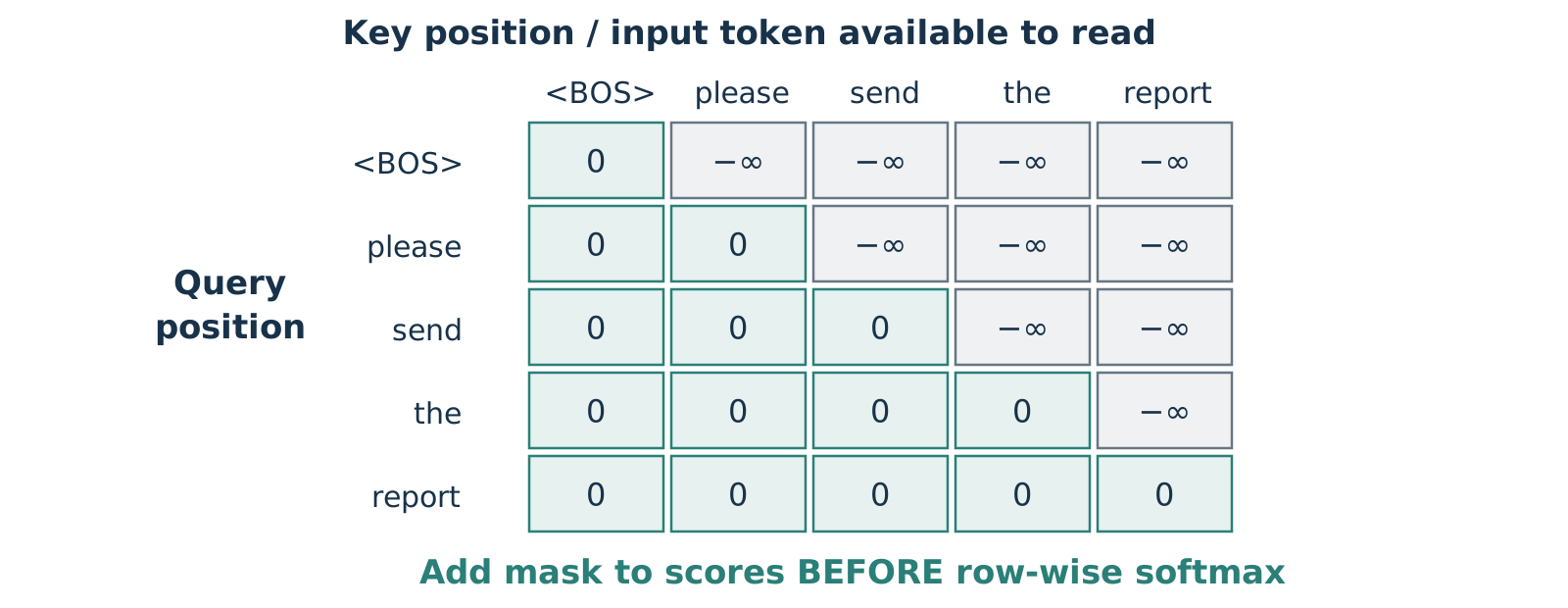
\[A=\operatorname{softmax}_{\rm row}(S+M),\qquad Y=AV\]

Three minutes. Show the row for send: it may read BOS, please and send, but not the or report. The diagonal is allowed because input token w_predicts w_(+1). Negative infinity produces zero exponential. In the toy, appending a future score log 9 would give that future key weight 9/15; masking restores [1,2,3,0]/6. Mask after score computation but before normalization; merely zeroing probabilities afterward would leave row sums wrong unless renormalized. Every meaningful query must have at least one allowed key. [Sources] source:vaswani-attention-2017.

Position tells the model where a matching token occurred

Arc 6: Attention and position

1. Combine values using query–key matches.
2. Restrict future-token access for next-token prediction.
3. Locate tokens with position information.

Then combine information in several learned subspaces.

Thirty seconds. Masks say which positions are allowed. Position features describe where content occurred. These are different roles; a causal mask does not replace an explicit position mechanism in the architectures we are teaching.

Self-attention without positions is permutation equivariant

For any permutation matrix \(P\), with no mask or positional encoding:

\[\operatorname{SA}(PX)=P\operatorname{SA}(X)\]

The outputs are the same, just reordered.

Input rows	Output rows
Item A · Item B · Item C	\(\boldsymbol{y}_A\) · \(\boldsymbol{y}_B\) · \(\boldsymbol{y}_C\)
Item C · Item A · Item B	\(\boldsymbol{y}_C\) · \(\boldsymbol{y}_A\) · \(\boldsymbol{y}_B\)

Useful for an unordered set: changing the storage order should not change what each item means.

Three minutes. P is a permutation matrix here, not the later matrix of position features. It reorders rows without changing their content. Equivariance means outputs reorder; it does not mean the output array stays identical (invariance). Example: contextualize objects in a bag or points in a point cloud whose spatial features travel with each point. Arbitrary enumeration should not change the per-item result. A symmetric pooling operation could then produce a permutation-invariant set summary. Proof sketch: Q,K,V become PQ,PK,PV; scores become PSP transpose; row softmax gives PAP transpose; multiplying by PV gives PAV. Shared projections and no index-dependent operations are essential. This is the deterministic attention operation, with dropout absent. [Sources] source:vaswani-attention-2017, section 3.2; the permutation identity is a direct algebraic consequence of the displayed operator.

A sequence needs order beyond an unordered collection

Same words, different order	Requested action
Send the report before the slides.	Report first, slides second.
Send the slides before the report.	Slides first, report second.

Focus on report: its relationship to before has changed.

Without a mask or positions, self-attention gives report the same output vector in both sentences—just in a different row.

We want token representations to reflect order-dependent relationships.

Two minutes. A content-identical token carries the same contextual output after a permutation when no positions or masks are used. The array still has an order, and an order-sensitive downstream operation could use that array order, so do not claim that every possible model containing attention is unable to distinguish these sentences. The limitation is that this self-attention operation does not contextualize a token differently because it moved earlier or later. We want the sequence architecture itself to use those relationships. [Sources] source:vaswani-attention-2017, section 3.5.