Attention, Transformers, and Generation
ECE 57000 — October 30, 2026
Attention chooses content and allowed context
- Learned queries and keys score matches; row softmax weights the value vectors.
- A causal mask excludes future inputs before softmax; training can compute every allowed output together.
- Unmasked attention without position signals reorders its outputs when inputs are reordered.
Today: represent order explicitly, then assemble a complete transformer.
Column vectors become transposed rows in a sequence matrix
\[X=\begin{bmatrix}\boldsymbol{x}_1^{\mathsf T}\\\vdots\\\boldsymbol{x}_L^{\mathsf T}\end{bmatrix},\qquad
\boldsymbol{q}_\ell=W_Q\boldsymbol{x}_\ell,\qquad Q=XW_Q^{\mathsf T}\]
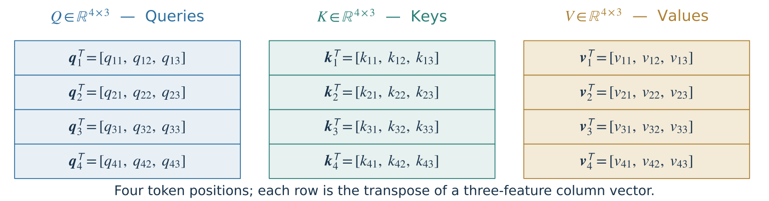
Likewise \(K=XW_K^{\mathsf T}\) and \(V=XW_V^{\mathsf T}\). Example: four tokens, three features per vector.
![Q, K and V are each four by three. Each colored row contains the transpose of a column query, key or value vector and its three scalar entries.]()
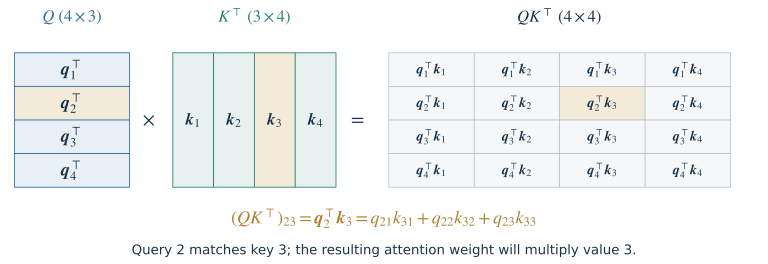
Each query–key inner product fills one score-matrix entry
![A four-by-three Q with query2 highlighted multiplies a three-by-four K transpose with key3 highlighted. The four-by-four product shows all sixteen q_i transpose k_j entries; entry2,3 is highlighted and expanded into three scalar products.]()
\[S=\frac{QK^{\mathsf T}}{\sqrt{d_k}},\qquad
A=\operatorname{softmax}_{\rm row}(S),\qquad
a_{\ell j}=\frac{e^{s_{\ell j}}}{\sum_{r=1}^{L}e^{s_{\ell r}}}\]
Dot products give scores; row softmax gives weights.
A sequence needs order beyond an unordered collection
| Send the report before the slides. |
Report first, slides second. |
| Send the slides before the report. |
Slides first, report second. |
Focus on report: its relationship to before has changed.
Without a mask or positions, self-attention gives report the same output vector in both sentences—just in a different row.
We want token representations to reflect order-dependent relationships.
Which change makes position explicit?
A causal attention layer already blocks future inputs.
Which change directly supplies each token’s absolute position?
A. Add a position vector to its embedding
B. Add another identical causal mask
C. Increase the number of attention heads
A. The mask controls access; a position vector explicitly represents location.
Causal masks restrict access; position signals describe location
A fixed causal mask breaks arbitrary permutation equivariance: reordering tokens changes which context they may read.
| Causal mask |
Which earlier/current inputs a query may access |
| Absolute position signal |
Where a token occurs in the sequence |
| Relative position signal |
How far apart two token positions are |
The mask does not explicitly encode token indices or pairwise offsets.
Next: add position features, or rotate query/key features using their positions.
Additive positions combine token features and location features
Look up the token’s embedding, then add a vector describing its position:
\[\boldsymbol{x}_\ell=E[w_\ell,:]^{\mathsf T}+\boldsymbol{p}_\ell,\qquad \boldsymbol{x}_\ell,\boldsymbol{p}_\ell\in\mathbb{R}^{d}\]
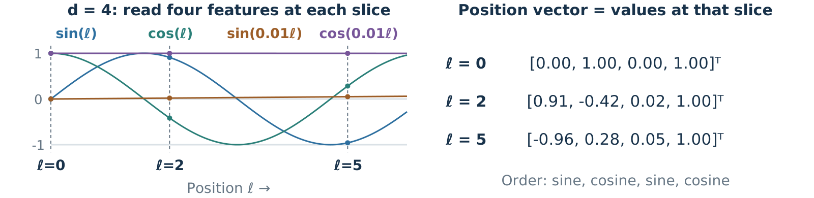
Fixed sinusoids: \(p_{\ell,2i}=\sin(\ell\omega_i)\), \(p_{\ell,2i+1}=\cos(\ell\omega_i)\), \(\omega_i=10000^{-2i/d}\).
Pair index \(i=0,\ldots,d/2-1\); even width \(d\).
![Four sinusoidal features for d=4. Vertical slices at positions 0, 2 and 5 give the complete position vectors printed beside the curves.]()
Same token “the” at positions 0 and 2: \(E[\text{the},:]^{\mathsf T}+\boldsymbol{p}_0\ne E[\text{the},:]^{\mathsf T}+\boldsymbol{p}_2\).
RoPE rotates query and key pairs by their positions
Split each query/key into 2-D feature pairs; rotate every pair by a position-dependent angle.
\[R(\alpha)=\begin{bmatrix}\cos\alpha&-\sin\alpha\\\sin\alpha&\cos\alpha\end{bmatrix},\qquad
\widetilde{\boldsymbol{q}}_\ell^{(i)}=R(\ell\theta_i)\boldsymbol{q}_\ell^{(i)}\]
\[[\underbrace{q_{\ell,0},q_{\ell,1}}_{\text{pair 0: }\ell\theta_0},\quad
\underbrace{q_{\ell,2},q_{\ell,3}}_{\text{pair 1: }\ell\theta_1},\quad\ldots]^{\mathsf T},
\qquad \theta_i=10000^{-2i/d_k}\]
Fast and slow pairs cover different distance scales. Keys use the same rotations.
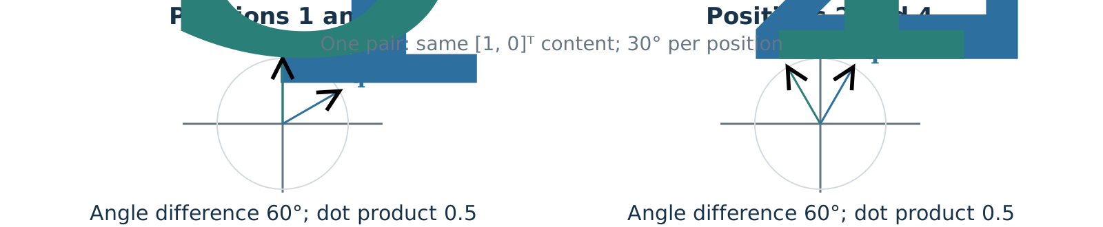
![One illustrative feature pair: query/key positions 1 and 3 versus 2 and 4. Rotating both by an extra 30 degrees preserves the 60-degree angle difference.]()
RoPE compares positions through angle differences
Moving both tokens one step rotates both arrows by the same extra angle: their angle difference stays the same.
\[s\theta_i-\ell\theta_i=(s-\ell)\theta_i,\qquad
(\widetilde{\boldsymbol{q}}_\ell^{(i)})^{\mathsf T}\widetilde{\boldsymbol{k}}_s^{(i)}
=(\boldsymbol{q}_\ell^{(i)})^{\mathsf T}R((s-\ell)\theta_i)\boldsymbol{k}_s^{(i)}\]
The full dot product adds the matches from all feature pairs.
| Relative offset enters the query–key match directly |
Same separation gives the same positional comparison, with content held fixed. |
| Fixed rotations, no learned position table |
Few extra operations; no separate learned vector for every index. |
Used in Llama 2: RoPE is itself a positional encoding, an alternative to adding absolute position vectors.
Multiple heads learn different ways to combine context
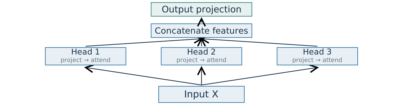
![The input at the bottom feeds three separate learned projection and attention heads. Their outputs concatenate along features and pass through an output projection.]()
\[Y=\operatorname{Concat}(Y_1,\ldots,Y_b)W_O^{\mathsf T}\]
Each head has its own query/key/value projections; every head obeys the allowed context.
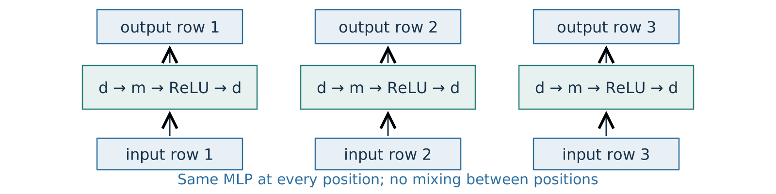
Next: combine attention with residual paths, normalization and a token-wise MLP.
Implementation detail: padding masks exclude absent tokens
Two messages share a batch:
| Message A |
please · send · the · report |
| Message B |
send · report · <PAD> · <PAD> |
- Attention key mask: padded positions cannot supply values to real queries.
- Loss mask: padded targets contribute no training loss.
A causal mask still applies within each real prefix.
A transformer combines context mixing and feature transformation
Transform features → preserve a residual path → normalize → stack blocks.
Keep the same task: use an email prefix to predict its next token.
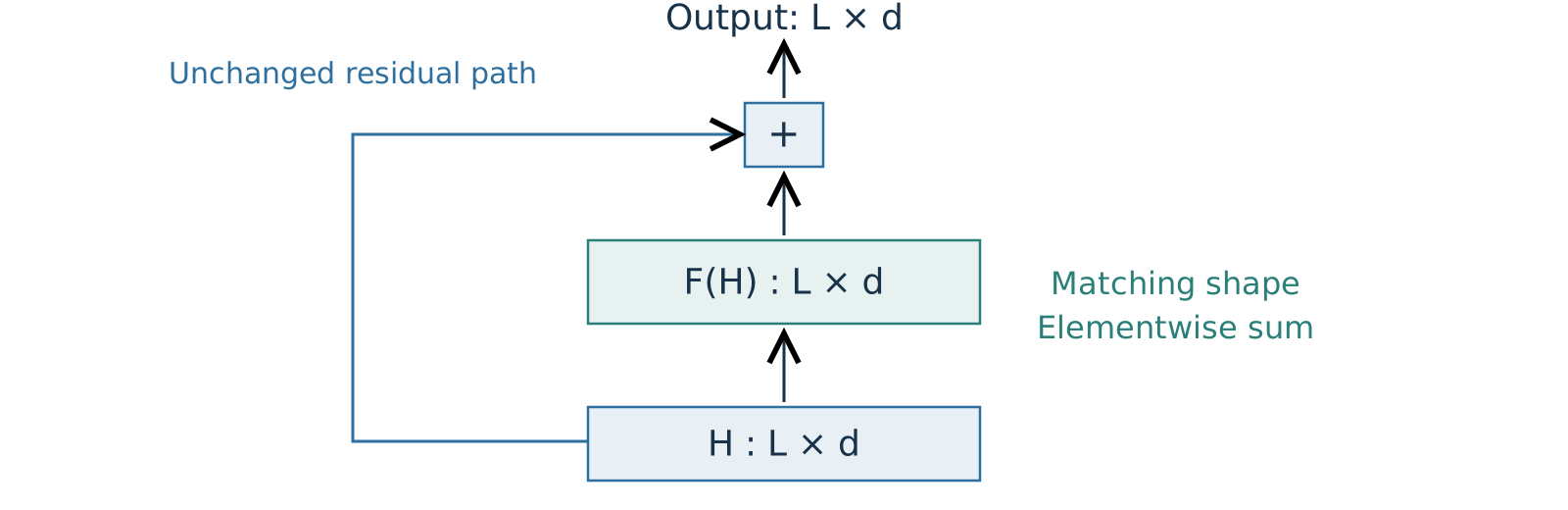
A residual path adds a learned update without changing the shape
![Reading upward, an L by d state branches into an unchanged bypass and a learned update F, also L by d. Elementwise addition returns L by d.]()
\[H_{\mathrm{out}}=H+F(H)\]
The attention output projection and the MLP’s last layer both return \(d\) features.
LayerNorm normalizes one token’s features at a time
Like BatchNorm: subtract a mean, divide by a standard deviation, then learn a scale and shift.
\[\mu_\ell=\frac1d\sum_{j=1}^{d}h_{\ell j},\qquad
\sigma_\ell^2=\frac1d\sum_{j=1}^{d}(h_{\ell j}-\mu_\ell)^2\]
\[\operatorname{LN}(\boldsymbol{h}_\ell)=\boldsymbol{\gamma}\odot
\frac{\boldsymbol{h}_\ell-\mu_\ell\boldsymbol{1}}
{\sqrt{\sigma_\ell^2+\epsilon}}+\boldsymbol{\beta}\]
- BatchNorm (CNN): one channel across batch examples and spatial locations.
- LayerNorm: one token across its \(d\) features—the last axis of
[B,L,d].
At evaluation, LayerNorm still uses that token’s statistics; BatchNorm usually uses running statistics.
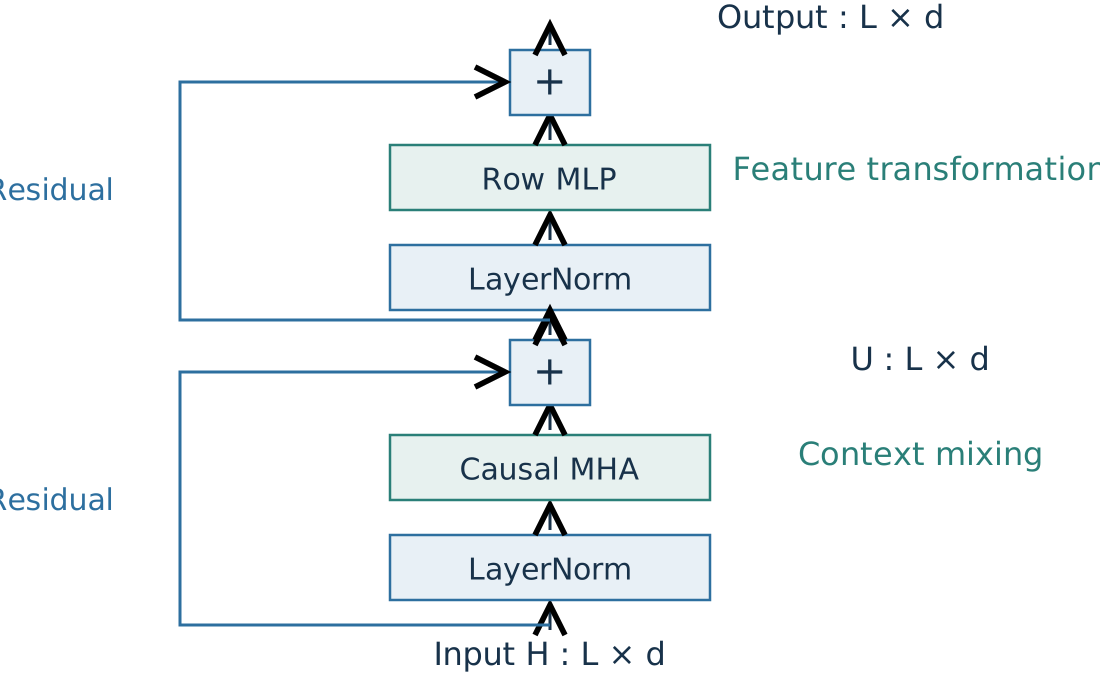
A pre-norm block adds two shape-preserving updates
\[U=H+\operatorname{MHA}_{\mathrm{causal}}(\operatorname{LN}_1(H))\] \[H_{\mathrm{out}}=U+\operatorname{MLP}(\operatorname{LN}_2(U))\]
Pre-norm is the usual modern LLM default. The original Transformer used post-norm.
| \(H+F(\operatorname{LN}(H))\) |
\(\operatorname{LN}(H+F(H))\) |
| Normalize before the branch. |
Normalize after addition. |
Pre-norm leaves the bypass untouched.
Stacked blocks turn token features into next-token logits
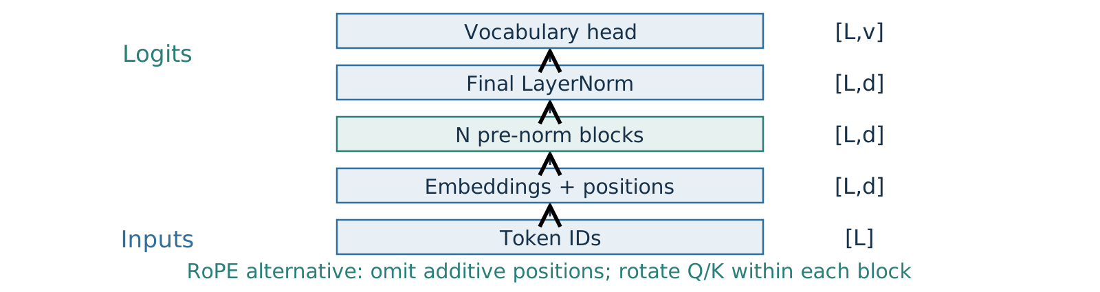
![Token IDs at the bottom enter learned embeddings plus additive positions, then N distinct pre-norm blocks, final LayerNorm, and a vocabulary head producing L by V logits. An alternative replaces additive positions with RoPE in every block's queries and keys.]()
\[H^{(0)}=E[w_{0:L},:]+P,\qquad
Y=\operatorname{LN}_{\mathrm{final}}(H^{(N)})W_{\mathrm{vocab}}^{\mathsf T}+\boldsymbol{1}\boldsymbol{c}^{\mathsf T}\]
\[H^{(N)}\in\mathbb{R}^{L\times d},\qquad
W_{\mathrm{vocab}}\in\mathbb{R}^{v\times d},\qquad Y\in\mathbb{R}^{L\times v}\]
Backpropagation follows different dependency graphs
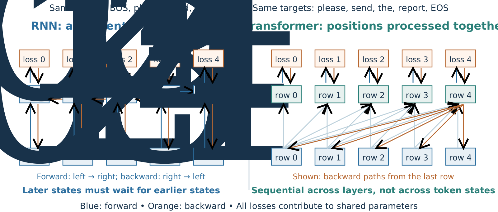
![The same five inputs and targets are used for both models. The RNN has a left-to-right hidden-state chain with reverse gradient arrows. A simplified transformer layer has causal connections between two rows of token states; the last row's reverse paths fan back to all allowed earlier positions. All losses contribute gradients.]()
Transformer benefit: parallel work across positions in forward and backward computation.
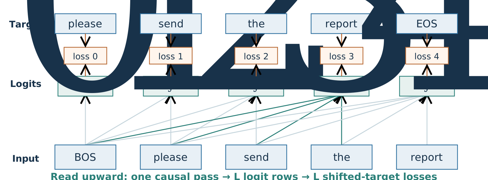
Can one forward pass score all shifted targets?
The training batch contains each full email.
Which model change would let an early prediction read its future target?
A. Compute all causal output rows together
B. Normalize each token over its own features
C. Remove the causal attention mask
C. Parallel computation is valid when every path respects the allowed prefix.
A causal decoder is the common decoder-only LLM architecture
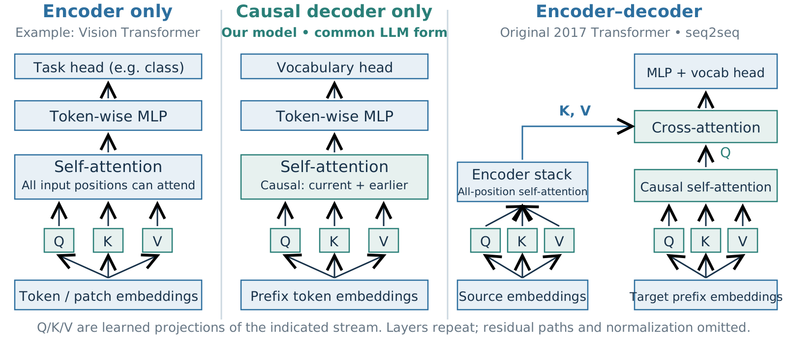
![Three upward architecture diagrams. Encoder-only uses Q/K/V from all input embeddings and a task head, with ViT as an example. Our causal decoder uses Q/K/V from the prefix with causal self-attention. The original 2017 encoder–decoder has source self-attention, target causal self-attention, and cross-attention with Q from target and K/V from source. Residual and normalization paths are omitted.]()
Our email model is a causal decoder. Other tasks can use different information paths and heads.
From Prediction to Generation
David I. Inouye
Dynamic Content · Last Updated: October 30, 2026
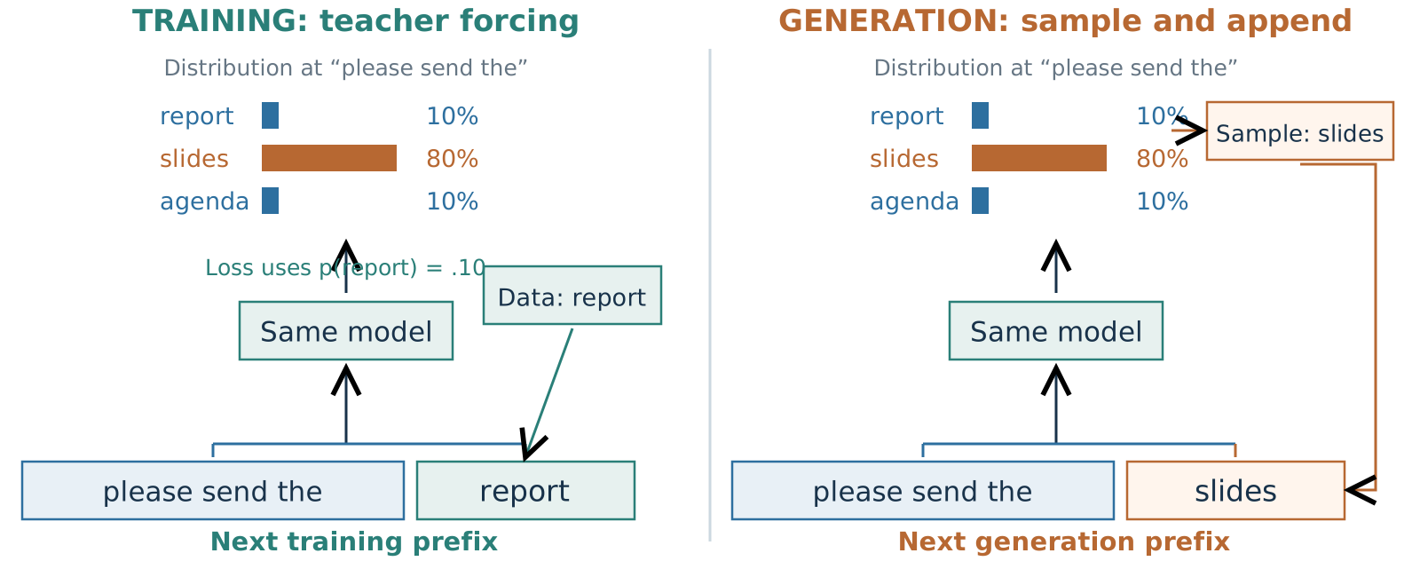
A next-token model becomes a generator through repeated feedback
Factorize → choose a token → append → repeat → evaluate.
We have an email-prefix model. Now we must choose a continuation and decide when to stop.
A sequence probability is a product of conditional probabilities
For a fixed prompt \(c\) and continuation tokens \(w_1,\ldots,w_L\):
\[p_\theta(w_{1:L}\mid c)=\prod_{\ell=1}^{L}p_\theta(w_\ell\mid c,w_{<\ell}).\]
Synthetic token example:
\[p_\theta(\text{report, today, EOS}\mid \text{please send the})\] \[=p_\theta(\text{report}\mid c)\;p_\theta(\text{today}\mid c,\text{report})\;p_\theta(\text{EOS}\mid c,\text{report,today}).\]
Taking negative logs turns the product into the sum used in next-token training.
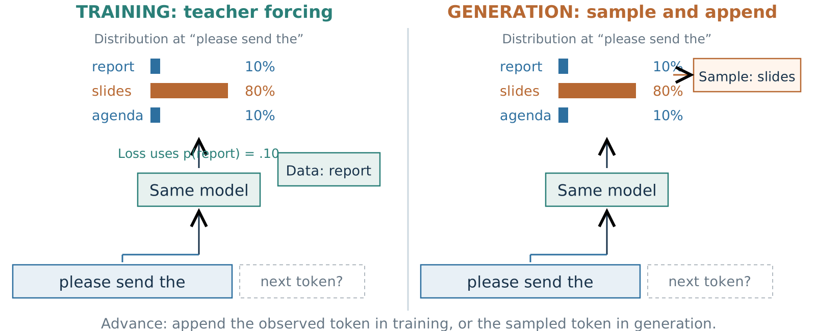
Teacher forcing uses the true prefix—even when the model is wrong
Training prefixes are all known in advance → a causal transformer can process them together.