Generation, Transformer Systems, and Empirical Comparison

ECE 57000 — November 2, 2026

David I. Inouye

Known prefixes allow parallel training; generation needs feedback

• A causal transformer mixes allowed context, then transforms each token’s features.
• With observed inputs, one pass predicts all shifted targets; the causal mask prevents future access.
• A sequence probability multiplies next-token conditionals; generation must choose each new token.

Today: choose and feed back tokens, then account for inference time and memory.

Two minutes. October 30 finished attention/position and transformer assembly, then introduced the probability chain rule and teacher forcing. Repeat the exact final teacher-forcing slide next, including its feedback reveal. Known prefixes permit parallel causal transformer training; they do not remove an RNN’s recurrent dependency. Attention and token-wise MLPs play different mixing roles. Avoid repeating the positional derivations or suggesting that parallelism guarantees a particular runtime speedup. [Sources] source:vaswani-attention-2017; source:d2l-rnn.

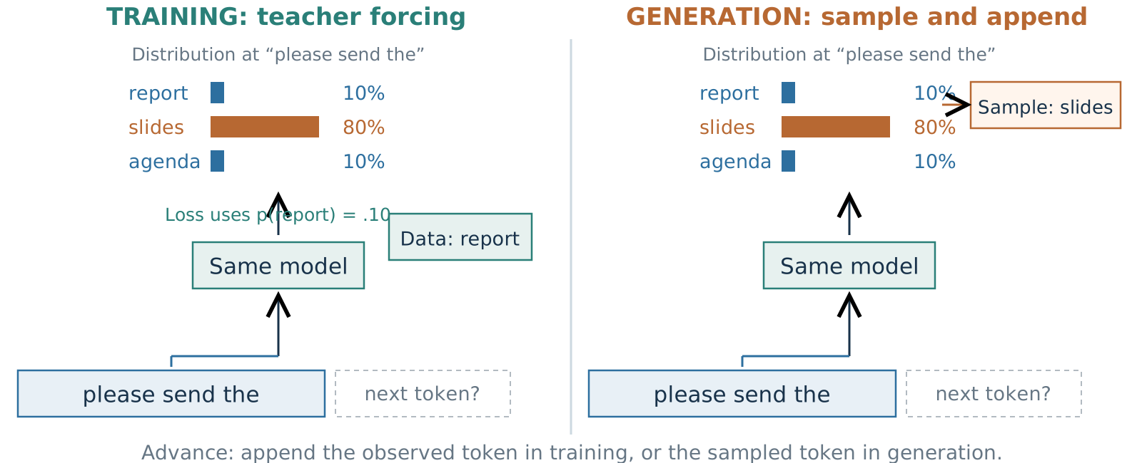
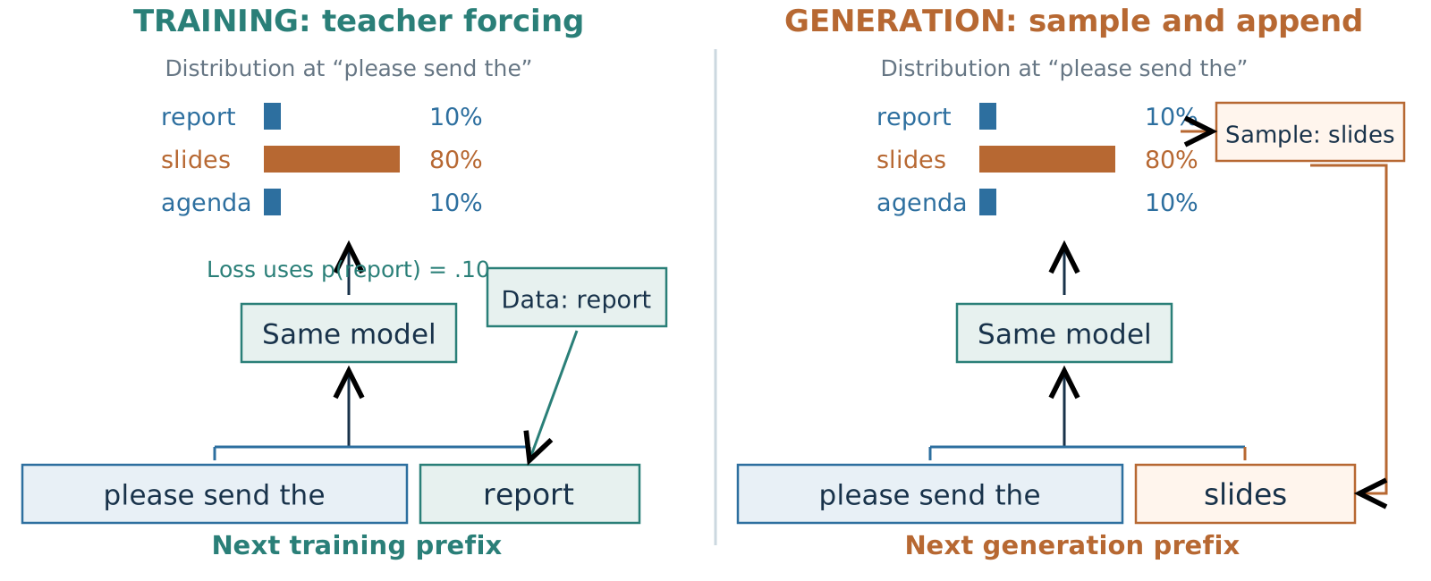
Teacher forcing uses the true prefix—even when the model is wrong

Training prefixes are all known in advance → a causal transformer can process them together.

Four minutes. Advance once to append the new token at the end of each bottom prefix row; both model blocks stay fixed. Bars remain labeled as the distribution at the original prefix. This is a comparison of conditioning rules, not a claim that training runs these prefixes sequentially. Synthetic probabilities, not measured model outputs. The observed email is “please send the report …”. At the prefix “please send the”, report is the supervised target even though slides has much higher model probability. Cross-entropy penalizes the low probability assigned to report. The next training task conditions on “… the report” regardless of the model’s distribution; no sample or argmax is fed into that task. This use of observed preceding tokens is teacher forcing. Both prefixes are known before the forward pass; the causal transformer computes their output rows together. An RNN can also use teacher forcing but still has a recurrent hidden-state dependency: known inputs are necessary here, not sufficient for position parallelism in every architecture.

At generation there is no observed next token to insert. One categorical draw selects slides in the pictured example; it is not guaranteed to select the most probable token. Append the draw, then evaluate the next distribution. Parameters stay fixed. “True” means the observed training sequence, not a guarantee that its statements are factually true. This original redraw follows the ground-truth-versus-feedback teaching idea in the prior course’s teacher-forcing illustration. [Sources] source:vaswani-attention-2017; source:d2l-rnn.

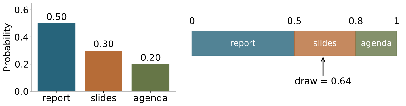
Greedy choice takes the largest bar; sampling uses all the bars

Greedy: choose \(\arg\max_j p_j\). Categorical sampling: choose token \(j\) with probability \(p_j\).

Three minutes. The probability vector is a column. Use a single uniform draw and cumulative probability intervals to explain categorical sampling before introducing temperature. The shown draw 0.64 selects slides. Repeated independent draws at the SAME prefix have these frequencies in expectation; a generated sentence changes the prefix after every draw. Greedy is deterministic given logits and a tie rule. Greedy does not necessarily maximize the full-sequence probability: in a synthetic two-step example, first-choice probabilities .6/.4 followed by best conditional probabilities .5/.9 yield .30/.36. The locally best first choice loses globally. Keep this as a short spoken counterexample rather than another table. [Sources] source:leviathan-speculative-decoding-2023, section 2.2.

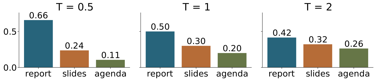
Temperature changes how concentrated the choices are

For the vocabulary-logit column \(\boldsymbol z\) and temperature \(T>0\):

\[p_{T,j}=\frac{\exp(z_j/T)}{\sum_{k=1}^{v}\exp(z_k/T)}.\]

Same model and prefix. Different sampling distribution.

Three minutes. Use z=log([.5,.3,.2]), so T=1 reproduces the preceding distribution. Temperature preserves logit ordering for positive T. As T approaches zero, mass concentrates on maximal logits; use a tie rule when comparing this limit with greedy. T=0 is not valid in this formula. Larger T flattens a finite-logit distribution toward uniform. Temperature does not supply evidence, retrieve facts, or retrain weights. [Sources] source:leviathan-speculative-decoding-2023, section 2.2. The plot is an original arithmetic example.

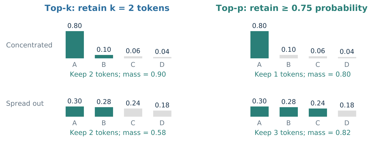
Top-k fixes the count; top-p sets a mass threshold

Keep the selected tokens → renormalize their probabilities → sample.

Top-p (nucleus sampling) keeps the smallest highest-probability set reaching the threshold.

Four minutes. A–D are synthetic token labels, sorted by current probability. Gray bars are removed; teal bars remain eligible. Top-k keeps the k most probable tokens (with a deterministic tie rule in this illustration). Top-p keeps a variable count: sort probabilities, take the shortest prefix whose cumulative mass is at least p, including the token that crosses the threshold. Here p=.75 needs one token for the concentrated distribution and three for the spread-out one. The retained mass can exceed p. Divide each retained probability by retained mass; then draw categorically. Top-k does NOT sample uniformly among k tokens, and top-p does NOT require each token individually to have probability above p. Both remove tail choices without changing weights. They can be combined with temperature; specify the order, for example temperature then filtering then normalization then sampling. Real-library tie and minimum-token conventions can differ. [Sources] source:huggingface-generation-methods-2020, Top-K Sampling and Top-p (nucleus) sampling.

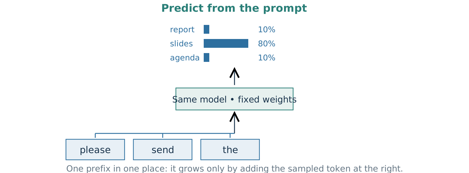
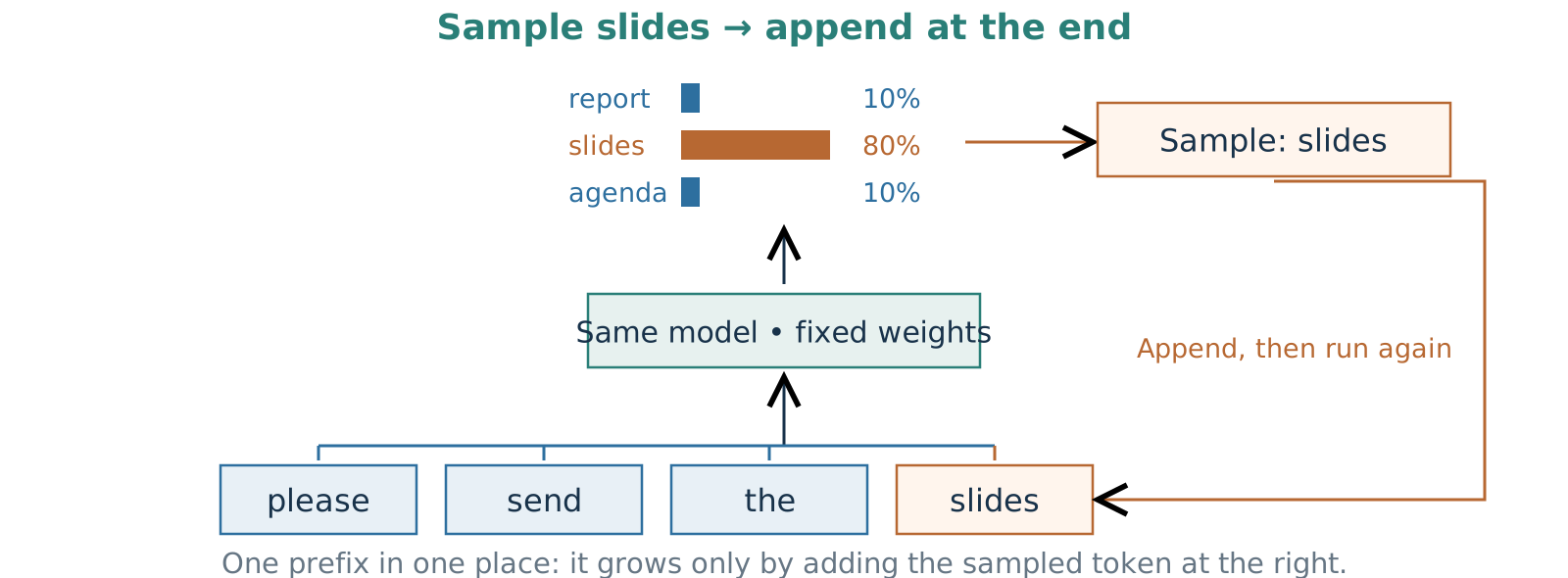
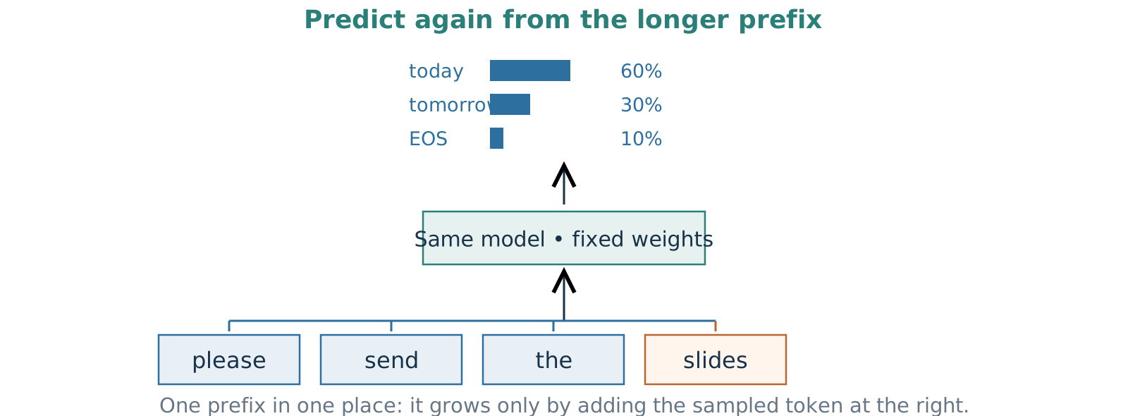
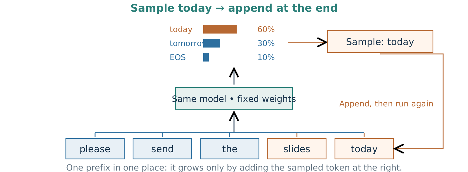
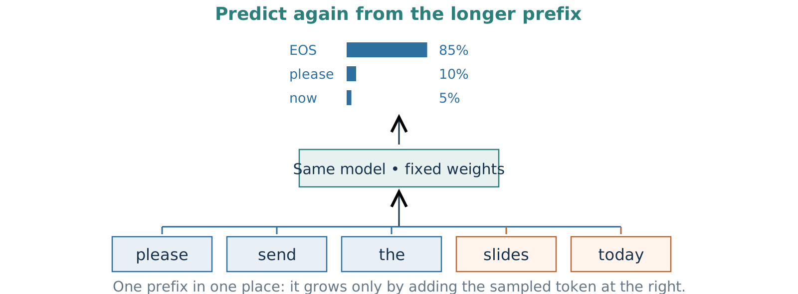
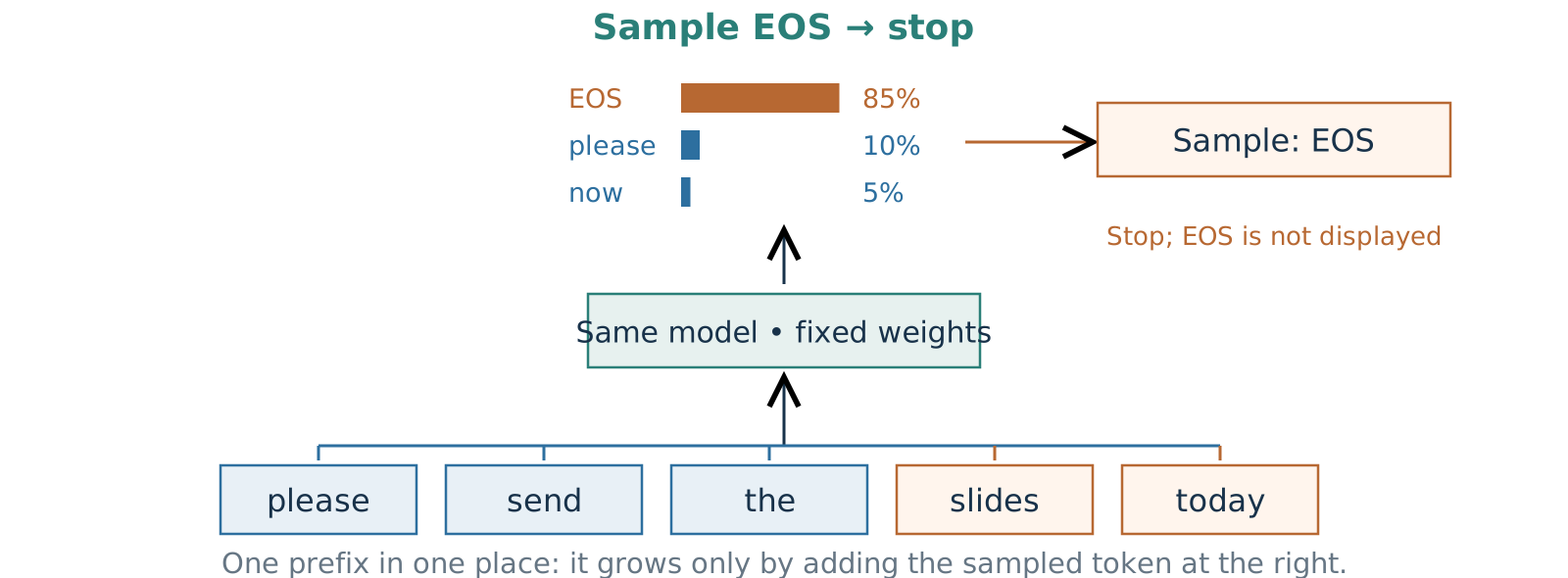
Generation samples, appends, and runs the model again

Stop on EOS, a new-token cap, or the model’s context limit.

Three minutes. Advance five times through six frames. The model block and initial three token boxes never move. First compute probabilities; then sample slides and append its box at the right. Run the same model on the longer prefix, sample today and append its box. Finally run again, sample EOS, and stop. Sampling/append frames retain the previous distribution and explicitly precede the next model pass. EOS is not displayed as text. All probabilities and draws are synthetic. The same parameters are used on every pass. Each next prefix depends on the preceding draw; unlike teacher-forced training, future inputs are not available together. The example uses plain categorical sampling; the next comparison slide collects alternative choice rules. In real execution KV caching can reuse earlier computation while preserving this logical dependency. A length cap is needed because EOS need not be selected; stop before exceeding context capacity in this teaching loop. [Sources] source:d2l-rnn; source:huggingface-kv-cache-4-57-1.

Can we change how a trained model generates?

We switch a trained model from greedy decoding to top-p sampling.

What must change?

A. The model’s learned weights

B. The rule for choosing the next token

C. The causal attention mask

B. No retraining needed. We sample from the retained tokens instead of always taking the largest probability.

Three minutes including voting. This follows the sample–append loop and leads directly into the decoding comparison. For a fixed prefix and deterministic model evaluation, the model produces the same logits under either rule. Greedy takes the maximum; top-p keeps the highest-probability tokens reaching the chosen cumulative mass, renormalizes, and samples. The weights and causal mask stay fixed. A different chosen token changes the subsequent prefix, so later model probabilities can differ even though the weights do not. A and C test whether students confuse changing the inference rule with changing the trained predictor or its context access. The previous factuality caveat remains in the temperature and final comparison notes. [Sources] source:huggingface-generation-methods-2020.

The same trained model supports different generation choices

Choice	How it chooses the next token	Main control
Greedy	Take the largest probability	Deterministic local choice
Categorical sampling	Draw from the full distribution	Random variation
Temperature sampling	Rescale logits by \(1/T\), then sample	Concentration
Top-k sampling	Keep \(k\) highest-probability tokens, renormalize, sample	Fixed candidate count
Top-p sampling	Keep the smallest set reaching mass \(p\), renormalize, sample	Adaptive candidate count

Inference choices: same weights and training; different generated outputs.

Evaluate the model + decoding rule for the task. Temperature and filters can be combined.

Three minutes. These choices are made during inference; changing them does not require retraining the baseline model. Their consequences are not independent of the model’s learned distribution or the task, so avoid a claim that one rule universally improves performance. Generation quality, diversity, repetition and task success may change. Temperature is a distribution transformation that can precede a top-k or top-p filter, not a mutually exclusive architecture choice. Greedy with a fixed tie rule is deterministic for fixed logits; sampling introduces randomness. These are the procedures covered here, not an exhaustive decoding taxonomy.

Preserve the evidence boundary: the email RNN/bigram comparison remains measured, while this transformer’s continuation quality and paired-prefix diagnostics remain unmeasured. Synthetic distributions do not supply empirical quality claims. Comparable held-out log loss needs the same split and tokenization; useful suggestions require task-specific evidence, and low-temperature agreement is not factual support. Next, the systems section asks how the same model and generation process fit memory and latency budgets. [Sources] source:huggingface-generation-methods-2020; source:leviathan-speculative-decoding-2023; source:aeslc-2019; source:chen-smart-compose-2019.

Serving and Training a Transformer

David I. Inouye

Dynamic Content · Last Updated: November 2, 2026

Serving a model means managing user latency and request memory

Prefill and decode → why K/V can be reused → memory → context growth.

Then: data movement, throughput and inference diagnosis.

First serve the trained model; afterward, consider training it.

Thirty seconds. Keep all inference concerns together before the separate training-memory section. The task and model remain unchanged; focus on where time and memory go.

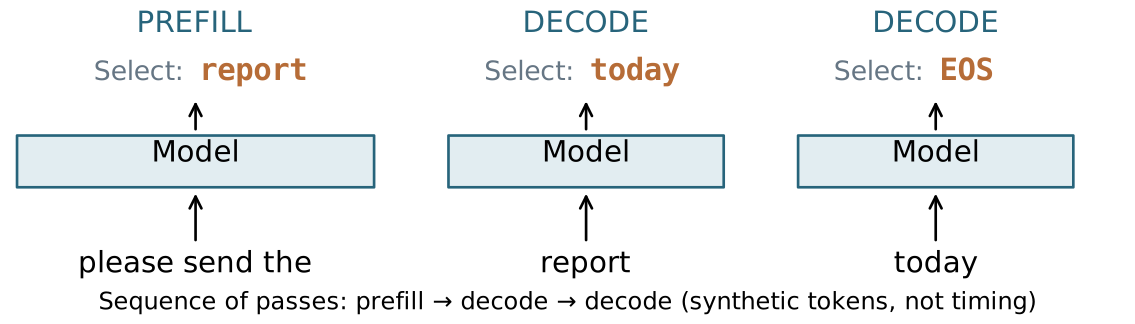
Prefill reads the prompt; decode extends it one token at a time

Work	Inputs already known	User-facing measure
Prefill	All prompt tokens	Time to first token
Decode	One new input token per step	Time per subsequent token

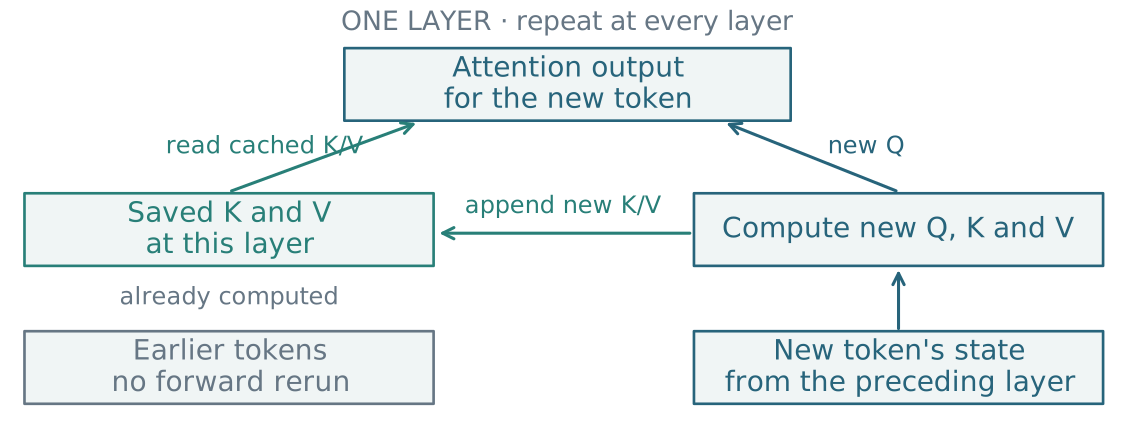
Prefill saves per-layer keys and values; each decode step reuses and extends them.

Three minutes. Prefill computes representations and cache entries for the prompt; the final prompt row supplies logits for the first generated token. The first generated token is then processed by decode to produce the second. Distinguish computing a token’s representation from selecting it. Training also knows all input tokens and can score causally shifted targets in parallel, but adds backward computation and optimizer updates. Time to first token can include queuing, tokenization and other overhead; it is not identical to kernel prefill time. Diagram widths show dependency stages, not measured time. [Sources] source:huggingface-kv-cache-4-57-1.

Earlier tokens stay fixed; attention needs only their keys and values

• Causal masking: appending a token cannot change earlier token states.
• Attention mixes tokens; MLPs, normalization and residual paths act within each token.

Keep old K/V at every layer; discard old queries and other intermediate states.

Five minutes. This explanation applies to the standard causal transformer already taught, with token-wise normalization and MLPs, fixed weights, unchanged prefix/positions and deterministic inference. At a layer, the only input-dependent route from earlier tokens into the new token is attention, through their keys and values. Earlier queries were used for earlier outputs; they are not needed for the new row. Earlier MLP outputs were needed to construct later-layer caches during prefill, but need not all be stored once the per-layer K/V are available. Never imply only the first layer is cached. The new token still executes the whole stack, including MLPs; caching avoids rerunning the old tokens, not reading their K/V. At one head: a_l = softmax(K_1:l q_l / sqrt(d_k)), o_l = V_1:l^T a_l, with column vectors and transposed rows in K/V. Append the new token’s K/V before its causal attention so it can attend to itself. RoPE keys retain their original position rotation. Edits to the prefix, reassigned positions or changed weights can invalidate cache entries. Training backward and nonstandard cross-token operators are outside this reuse claim. [Sources] source:huggingface-kv-cache-4-57-1; source:vaswani-attention-2017.

Inference keeps weights and K/V, plus temporary workspace

Memory term	Why it stays or grows
Model weights	Shared across requests; size depends on parameters and precision
K/V at every layer	Retained for later tokens; grows with prefix length and active requests
Temporary activations/workspace	Needed for current computations; reused or freed afterward

We cache the history attention will read—not every activation produced for that history.

Three minutes. The K/V explanation now comes before this ledger. Ordinary inference disables gradient recording and has no optimizer state. It still allocates Q, attention intermediates, MLP intermediates and workspace while executing the new token or prefill batch; these need not persist as the entire prefix’s activation history. Weights are model state, not token cache. Static implementations may preallocate cache capacity; shared-prefix implementations may share entries. KV caching trades persistent memory for less repeated prefix computation. [Sources] source:huggingface-kv-cache-4-57-1.

A longer context grows both the cache and the attention work

Quantity being counted	If context length doubles: \(L\rightarrow 2L\)
Compute: dense attention over a full prompt	About 4× as many query–key pairs
Compute: cached attention for one new token	About 2× as many query–key pairs
Memory: persistent K/V cache	2× as many stored K/V entries

Fixed model, precision and request count. Operation counts are not measured latency.

Conventional multi-head cache bytes \(\approx 2NBLdb\).

Synthetic example: \(N=12\) layers, \(B=1\), \(L=1024\), \(d=512\), \(b=2\) bytes → 24 MiB.

Three minutes. The leading 2 counts keys and values; N is layers, B active batch size, d total width across conventional heads and b bytes per entry. The arithmetic gives 25,165,824 bytes =24 MiB, excluding overhead. Grouped-query attention changes cache width and is outside this example. Dense attention’s pairwise work is quadratic; causal masking changes constants. A cached new query still reads all allowed keys/values. Do not equate attention work with total transformer runtime: projections, MLPs, memory traffic and batching also matter. Nor does quadratic pair count require materializing a full score array; that distinction motivates FlashAttention next. [Sources] source:huggingface-kv-cache-4-57-1; source:dao-flashattention-2022.

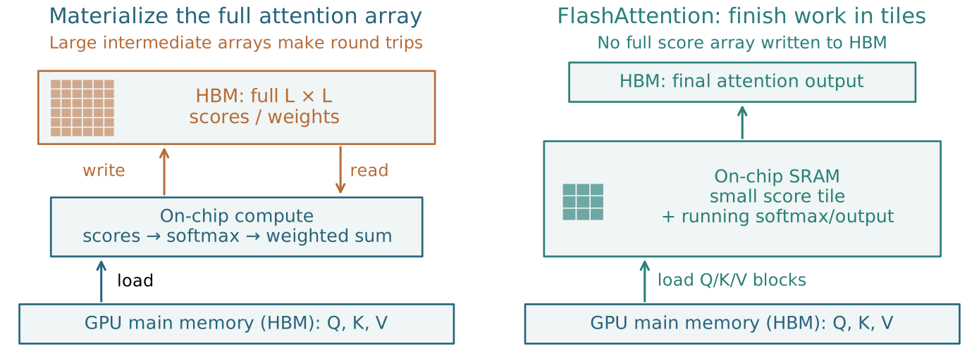
Fewer memory transfers can make the same attention faster

Same dense attention; fewer large memory round trips.

Tiling reduces intermediate storage and traffic; the pairwise arithmetic remains quadratic.

Three minutes. Connect to the previous context-scaling table: quadratic pairwise work does not require storing every pair score at once. FlashAttention tiles Q/K/V and maintains the normalization needed to combine blocks into the same mathematical attention result. Floating-point evaluation order can change rounding; exact does not promise bitwise equality. The original dense algorithm still performs quadratic pairwise arithmetic at fixed width. Its block-sparse extension is a separate approximation, not the claim here. Focus here on forward attention during prompt prefill. The same algorithm also supports training; its backward recomputation belongs to the later training discussion. Do not quote a universal speedup or assume every transformer phase is memory-bound. [Sources] source:dao-flashattention-2022, sections 1–3.

Higher throughput need not mean a faster response for each user

Measure	Main dependencies—and why
Time to first token	Queue/load + prompt length: wait for service, then prefill the prompt
Time per subsequent token	Model size + context + active batch: each step reads weights/K/V and computes the new token
Aggregate output tokens/sec	Batch size + hardware utilization: process several requests together to share weight access and parallel work

Larger batches can raise throughput while adding queueing, cache memory and per-step work.

More output tokens mean more sequential decode steps—and a longer total response time.

Three minutes. Batching lets multiple requests share a model pass, potentially improving hardware utilization and amortizing weight access. Each request still has its own prefix/cache; the cache ledger scales with active batch size. Waiting to assemble a batch can add queueing delay. These are possible tradeoffs, not a claim that every batching implementation makes every latency measure worse. A service can improve aggregate tokens/sec without improving one user’s time to first token or inter-token delay. Hardware, prompt lengths, output lengths and offered load must be comparable; no benchmark or measured speedup is asserted here. Low-batch decode is often constrained by memory traffic, but bottlenecks vary. [Sources] source:huggingface-kv-cache-4-57-1; source:dao-flashattention-2022.

Which memory grows when the prompt grows?

Fixed weights and request count; cached inference now runs out of memory on longer prompts.

What should we inspect first?

A. Parameter gradients and optimizer state

B. KV cache and temporary activations

C. The number of learned weights

B. Prefix-dependent memory grows even though the model’s weights do not.

Compare task quality, user latency, throughput and peak memory before choosing a fix.

Three minutes including voting. A recalls gradient-based learning from Arc 5, but normal inference does not maintain parameter gradients or optimizer state. C confuses a fixed model with variable request state. B names the likely growing terms without claiming the cache is always the sole cause: measure the allocations. Reducing context or concurrency changes the service offered; an exact memory-efficient attention implementation changes intermediate storage, but does not eliminate persistent KV entries. Tie the diagnosis back to choosing an optimization for a measured bottleneck. Close the inference section by distinguishing architectural access, held-out prediction and practical task utility; the existing RNN/bigram experiment is measured, while this transformer has no trained comparison yet. [Sources] source:huggingface-kv-cache-4-57-1; source:dao-flashattention-2022; source:pytorch-activation-checkpointing-2025.

Training adds backward computation and parameter updates

Memory ledger → precision and recomputation → sharing state across GPUs.

Serving keeps weights fixed. Training must also compute gradients and update them.

Thirty seconds. Explicit switch in objective and workload. Inference prioritizes each user’s response and concurrent-request memory. Training prioritizes fitting the learning computation and reaching useful model quality within a compute/time budget. Fine-tuning also performs training, even when only some parameters are updated. Keep this section shorter than the inference section. [Sources] source:pytorch-activation-checkpointing-2025; source:pytorch-amp-recipe-2026.

Full fine-tuning can need far more memory than serving

Qwen3-8B: approximately 8.2 billion parameters. Illustrative full-parameter AdamW setup:

Stored arrays	Bytes / parameter	Approximate memory
16-bit weights used for computation	2	16.4 GB
FP32 master weights for updates	4	32.8 GB
FP32 gradients	4	32.8 GB
Two FP32 Adam moment arrays	8	65.6 GB
Training state subtotal	18	147.6 GB

Inference: 16.4 GB weights + K/V + workspace.
Training: 147.6 GB state + saved activations + workspace.

Four minutes. Decimal GB (10^9 bytes), not GiB. The official model card reports 8.2B total parameters; this is approximate parameter-count arithmetic, not a measured run. The inference comparison assumes weights stored directly at 16 bits and no FP32 master copy. The illustrative mixed-precision full-parameter training setup retains 16-bit compute weights, FP32 master weights, FP32 gradients and two FP32 Adam moments. That is 18 bytes per parameter, or 147.6 GB (about 137.5 GiB); compute weights alone are 16.4 GB (about 15.3 GiB). Training state here is nine times inference weight storage, not nine times total inference peak memory. Other implementations may use different parameter/gradient precision or avoid a separate copy; 16-bit gradients would reduce this example to 131.2 GB. Activations depend on sequence length, microbatch, checkpointing and implementation, so no universal number is asserted. Without sharding/offload this subtotal alone exceeds an 80-GB GPU. LoRA/QLoRA train a smaller parameter subset and have a different ledger; do not present 147.6 GB as their requirement. Normal teacher-forced training uses saved activations, not a persistent autoregressive generation cache. This motivates precision, checkpointing and ZeRO next. [Sources] source:qwen3-8b-model-card, Model Overview; source:hf-model-memory-4-57-1, Anatomy of Model’s Memory.

Training can save memory by changing precision or recomputing activations

Choice	What changes	What to check
Mixed precision	Use lower precision for suitable operations; retain higher precision where needed	Numerical stability, quality and runtime
Activation checkpointing	Save fewer intermediates; recompute them during backward	Peak memory versus extra computation

Neither removes weights, gradients, optimizer state, and activations all at once.

Choose the technique for the memory term that is limiting the run.

Four minutes. Recall the training memory ledger. Mixed precision is not a blanket conversion of every tensor to a smaller format: operations and stored states can use different precisions; some schemes retain full-precision parameter or optimizer copies. Reduced precision can alter numerical results; compare convergence and held-out quality. Gradient scaling is useful for some low-precision formats but is not needed by every format. Activation checkpointing saves boundary inputs and reruns selected forward regions when backward needs their intermediates; it does not mean saving a model file to disk. Recomputed regions must preserve the required behavior, including random-state handling. More aggressive low-bit inference quantization is a separate choice and also needs quality evaluation. Keep API and distributed-training details out of this conceptual comparison. [Sources] source:pytorch-amp-recipe-2026; source:pytorch-activation-checkpointing-2025.

ZeRO reduces duplicated training state across GPUs

Ordinary data parallelism trains on different examples with a model replica on each GPU.

ZeRO (Zero Redundancy Optimizer) partitions state among those GPUs:

Stage	State partitioned across GPUs, cumulatively
1	Optimizer state
2	Optimizer state + gradients
3	Optimizer state + gradients + parameters

Less state stored per GPU; communication supplies the pieces when needed.

Three minutes, recognition-level only. Data-parallel workers contribute to training the same model using different examples; they must synchronize information for consistent updates. ZeRO avoids keeping every training-state array fully replicated on every worker. At stage 3 parameters are gathered as needed for computation and then repartitioned. This is not activation checkpointing and does not by itself eliminate activation/workspace memory. Communication, temporary gathered tensors and hardware affect the practical tradeoff; do not claim total memory divides exactly by GPU count or promise a speedup. No API/configuration, offload taxonomy or distributed-training derivation. The stages are cumulative. Close with three different levers: precision changes representation, checkpointing recomputes activations, ZeRO partitions duplicated state. [Sources] source:deepspeed-zero-tutorial-2026, ZeRO Overview.

Serving and training optimize different system outcomes

	Serving an LLM	Training / fine-tuning an LLM
Goal	Useful responses at acceptable latency, throughput and cost	Reach useful model quality within a compute/time budget
Memory	Weights + per-request K/V + workspace	Weights + gradients + optimizer state + saved activations
Levers	Cache K/V; manage context and batching; reduce attention traffic	Mixed precision; recompute activations; shard state with ZeRO

Identify the limiting resource, change the relevant term, then recheck quality and performance.

Two minutes. Summarize the whole systems section before moving to Arc 7. These are emphases, not exclusive technique lists: efficient attention and lower precision can help both serving and training. Caching reuses fixed history; checkpointing recomputes intermediates for backward; ZeRO shares state across workers. Each shifts memory, compute, communication or numerical behavior. Measure comparable workloads, including prompt/output length and offered load for serving, and learning progress as well as steps/second for training. A smaller allocation or faster kernel alone does not prove a better end-to-end system. [Sources] source:huggingface-kv-cache-4-57-1; source:dao-flashattention-2022; source:pytorch-amp-recipe-2026; source:pytorch-activation-checkpointing-2025; source:deepspeed-zero-tutorial-2026.

On short email prefixes, both models improve on the bigram

Return to email completion: same grouped split, 4,000-token vocabulary and 64-token cap.

Model	Test loss ↓ (nats/token)	Exact next-token accuracy ↑
Bigram	4.840	18.9%
Simple RNN	4.454	23.3%
Small causal transformer	4.445	22.8%

For “please send the”, both rank “attached” first; this is a diagnostic, not a quality score.

One seed, eight epochs each; no decisive architecture winner from this experiment.

Three minutes. These are measured results, not synthetic values. Frozen AESLC body-completion protocol: 13,415 train, 1,769 validation and 1,604 test emails, grouped by normalized subjects/duplicate prefixes as proxies rather than verified thread IDs. Test scores cover 91,824 targets; 6.5% are UNK. Known-target accuracy is 21.830% RNN and 21.824% transformer, reinforcing that aggregate accuracy alone can obscure what changed. The RNN is one ReLU recurrent layer with embedding 64 and hidden 96 (659,552 parameters). The transformer has two pre-norm causal layers, width 64, four heads, FF width 256, learned absolute positions, no dropout and an untied vocabulary head (620,192 parameters). Both use FP32 CPU Adam, learning rate .002, batch 64, gradient clipping 1, and eight predeclared epochs; lowest validation NLL selects epoch 7 RNN and epoch 8 transformer. Equal epochs are not equal FLOPs or equal tuning effort. Test used only after selection. This is a single descriptive comparison, not a significance result, controlled architecture ablation or claim about long context/large modern models. Exact evidence: lectures/experiments/email-completion-v1/results.json and lectures/experiments/email-transformer-v1/results.json. [Sources] source:aeslc-2019; source:pytorch-rnn-2-7; source:vaswani-attention-2017.

The smaller parameter count did not give the smaller training-memory peak

Measured CPU probe: FP32 Adam, batch 64, length 64, vocabulary 4,000; five training steps.

Quantity	Simple RNN	Small transformer
Parameters	659,552	620,192
FP32 parameter storage	2.52 MiB	2.37 MiB
Peak process memory	548 MiB	630 MiB

Process memory includes activations, optimizer state, runtime and allocator overhead—not just weights.

This is CPU process memory, not GPU VRAM or a universal architecture ranking.

Three minutes. Each model ran in a fresh process with identical random integer input/target shapes for five full forward/backward/Adam updates. This isolates a shape-matched execution probe from differences in training history; it is not measured on the entire corpus and does not use learned checkpoints. On macOS, resource.getrusage(RUSAGE_SELF).ru_maxrss reports peak resident process bytes. Recorded values are 547.855 MiB RNN and 629.914 MiB transformer; show rounded values. Both include the Python/PyTorch process, weights, gradients, Adam moments, activations, workspaces and allocator behavior. The output logits alone have 64644000 FP32 entries, or 62.5 MiB, and further loss/backward allocations contribute. Do not assign the entire difference to attention without profiling allocations. No GPU benchmark, throughput advantage, multiple-seed uncertainty or asymptotic memory measurement is claimed. One measured configuration each. This complements the systems explanation: recurrent decode can retain a fixed-size hidden state while transformer K/V grows with context; that decode-state comparison is not what this training-memory table measures. Evidence and measurement code: email-transformer-v1/results.json and scripts/arc6_email_transformer.py. [Sources] source:aeslc-2019; source:pytorch-rnn-2-7; source:vaswani-attention-2017.

Learning to Reconstruct and Restore Images

Arc 7 · Image generation and evaluation

Vanilla autoencoders and denoising autoencoders

Thirty seconds. Arc 6 ended with the computation needed to generate sequences. We now return to images: what can we learn from an image when no class label is supplied? Reconstruction and restoration give two learning tasks before we introduce explicit generative sampling. This topic is the first part of Arc 7, not the entire generative-modeling arc.