Learning to Reconstruct and Generate Images

ECE 57000 — November 4, 2026

David I. Inouye

A model’s objective and its use need separate evidence

• Generation feeds selected tokens back; decoding choices change outputs without retraining.
• Serving and training have different memory costs; parameter count alone predicts neither.
• Our short-email comparison supported both learned models, without a decisive architecture winner.

Next: move from generating text to generating images, beginning with models that reconstruct an image.

Two minutes. November 2 completed Arc 6 and displayed only the AE/DAE title during closing questions. The opening title above carries that transition; begin with the first untaught orientation after this recap instead of repeating another title. Preserve the distinction between measured CPU process memory and an unprofiled explanation of its difference. No exam cutoff or policy is inferred from the recording. Reuse PCA, composed networks and squared-error loss; the new question is what the learning objective makes possible.

We will build from reconstructing images to generating new ones

We generated text one token at a time. Now we turn to images, starting with two simpler learning tasks.

1. Reconstruct an image: learn an encoder and decoder with an autoencoder. (Today)
2. Restore a corrupted image: train a denoising autoencoder to recover the clean image. (Today)
3. Make the mappings probabilistic: then add a generative model to develop VAEs.
4. Evaluate the results: compare image quality, diversity, usefulness and cost. (Later)

Thirty seconds. Reuse PCA from Arc 2 and composed neural networks from Arc 5. The AE, denoising AE, VAE and diffusion model will receive distinct explanations. Today’s diagrams are original schematics, not trained-model results. The systems-to-images transition changes the task, not the optimization machinery. Other image-generation families include adversarial generators (GANs) and autoregressive image models; name these for orientation, without adding full method units. Autoregression was taught in Arc 6 for text. [Sources] source:ho-ddpm-2020, introduction.

We will use handwritten digits and small color images as examples

• MNIST: trace a recognizable digit through encoding, corruption and reconstruction.
• CIFAR-10: compare models on 32 × 32 color images with varied objects and backgrounds.

Use the same data, evaluation protocol and declared compute budget for comparisons.

Two minutes. The six displayed images are the first six training records in the archived MNIST IDX file; no cherry-picking for a model. MNIST has 784 grayscale input features. CIFAR-10 has 3072 color input features and 50,000 training/10,000 test images; use a train/validation split for model selection and reserve its test set. CIFAR generator comparisons are planned, not measured yet. Use reconstruction criteria for reconstruction, and distributional quality/diversity plus cost for generation; a vanilla AE has no default sampler. Class labels can aid evaluation without serving as training targets for an unconditional model. [Sources] source:mnist-train-images; source:cifar10-dataset.

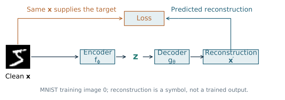
An autoencoder learns a code that supports reconstruction

\[\boldsymbol{z}=f_\phi(\boldsymbol{x}),\qquad \widehat{\boldsymbol{x}}=g_\theta(\boldsymbol{z})\]

Four minutes. AE means autoencoder. The running input is a 28 by 28 MNIST image (784 features), flattened into a vector for this notation; convolutional implementations can retain its spatial structure. Phi denotes encoder parameters and theta decoder parameters. The code is an internal learned representation. The target is the observed image, not a class label and not something created by the decoder. Both functions are learned together through the loss; do not confuse the decoder here with the causal transformer decoder. [Sources] source:goodfellow-autoencoders-2016, chapter 14 opening; source:mnist-train-images.

Reconstruction error trains both halves together

For images \(\boldsymbol{x}_i\in\mathbb{R}^d\), one choice is mean squared error:

\[\min_{\phi,\theta}\ \frac{1}{nd}\sum_{i=1}^{n} \left\|\boldsymbol{x}_i-g_\theta\!\left(f_\phi(\boldsymbol{x}_i)\right)\right\|_2^2.\]

• The image supplies its own reconstruction target.
• Backpropagation updates encoder and decoder parameters through the same loss.

A small pixel error measures reconstruction, not every property we care about.

Four minutes. Here n is the number of training images and d is the number of input features. The squared norm sums over image features, so division by nd gives an elementwise mean squared error. Use the already-taught optimization loop; no new backpropagation derivation. MSE is a modeling choice, not the definition of all AEs. Class labels are unnecessary for this objective, but data collection and choice of task still matter. Different images can have similar pixel losses while differing in usefulness. [Sources] source:goodfellow-autoencoders-2016, section 14.1.

Perfect copying can solve the loss without a useful code

If both functions can be the identity,

\[f(\boldsymbol{x})=\boldsymbol{x},\qquad g(\boldsymbol{z})=\boldsymbol{z} \quad\Longrightarrow\quad\|\boldsymbol{x}-g(f(\boldsymbol{x}))\|_2^2=0.\]

The reconstruction objective needs a constraint that makes learning useful structure worthwhile.

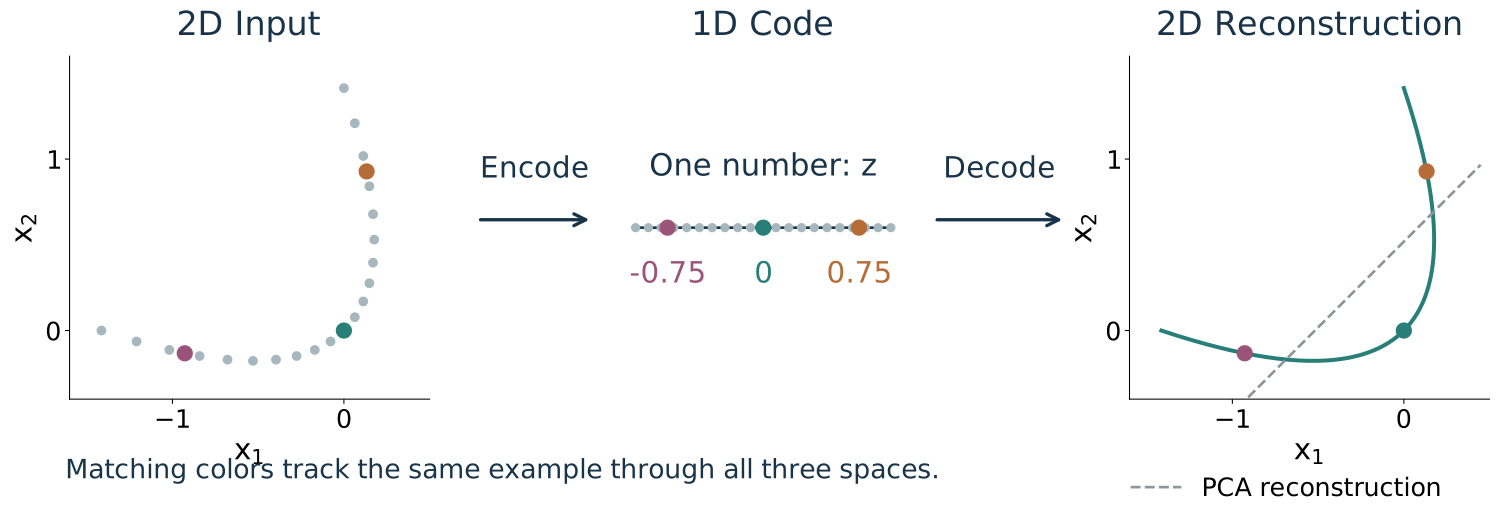
Our first choice: pass through a smaller code, \(\boldsymbol{z}\in\mathbb{R}^k\) with \(k<d\).

Three minutes. This is a mathematical counterexample, not an empirical claim that every unconstrained network learns identity. An undercomplete AE uses fewer code features than input features. Other constraints exist; sparse AEs are outside this arc’s core. A small code is an inductive bias, not a guarantee of semantics or generalization: a sufficiently flexible model can memorize a finite dataset. [Sources] source:goodfellow-autoencoders-2016, sections 14.1–14.2.

Remember: PCA encodes an input in fewer features and reconstructs it

We already know a linear encoder and decoder: PCA.

For a centered input \(\boldsymbol{x}\) and principal directions \(U_k\in\mathbb{R}^{d\times k}\):

\[\underbrace{\boldsymbol{z}=U_k^{\mathsf T}\boldsymbol{x}}_{\text{encode into }k\text{ features}}, \qquad\underbrace{\widehat{\boldsymbol{x}}=U_k\boldsymbol{z}}_{\text{decode back to }d\text{ features}}.\]

This gives an optimal rank-\(k\) linear reconstruction under squared error.

Learned linear AE factors can differ while producing the same reconstruction.

Four minutes. Recall the PCA geometry rather than repeat its proof. Center the data and add the mean back after reconstruction. A linear encoder/decoder with a k-dimensional bottleneck and globally minimized squared error can recover a principal-subspace reconstruction. The learned factors need not equal U transpose and U, nor provide ordered orthogonal code features; invertible changes of basis in the code can leave the product unchanged. Degenerate eigenvalues can make the optimum subspace nonunique. Do not promise gradient descent reaches the global optimum. [Sources] source:goodfellow-autoencoders-2016, section 14.1.

A nonlinear decoder maps a 1D code back to a 2D curve

Encode: \(z=(x_1+x_2)/\sqrt{2}\). \(\qquad\) Decode: \(\widehat{\boldsymbol{x}}=\frac{1}{\sqrt{2}}[z-z^2,\ z+z^2]^{\mathsf T}\).

The code combines both input features. Analytic example; no model was trained.

Four minutes. This is an analytic illustration; no neural network was trained. Start at the left: each input has two measured features, but the points lie on a curve parameterized by one number t in [-1,1]. Rotate the original [t,t²] column by 45 degrees to obtain x=[t-t²,t+t²]^T/sqrt(2). Neither raw feature alone is the displayed code. Follow one color through the middle: adding the two features cancels their quadratic terms, giving z=t. For z=.75, the input and reconstruction are approximately [.133,.928]^T. Follow the same color to the right: the decoder uses z and z² to recover both features. Exact reconstruction holds for this specified curve; arbitrary off-curve inputs need not reconstruct exactly. The dashed line is the rank-one PCA reconstruction of the same equally spaced samples, through their mean. Both methods use one scalar code; the nonlinear decoder can follow the curvature while the linear decoder is restricted to a line. The encoder here is deliberately linear: a nonlinear decoder alone suffices for this example, although learned AEs can make both functions nonlinear. This demonstrates representational possibility, not optimization success or generalization. An image AE needs held-out evaluation. [Sources] source:goodfellow-autoencoders-2016, section 14.1. Curve, functions and numerical trace are original analytic examples.

What does a small reconstruction error tell us?

An AE reconstructs held-out images accurately.

Which conclusion is supported?

A. Its codes separate all useful classes.

B. Its reconstructions preserve the measured image features well.

C. Random Gaussian codes produce realistic images.

B. Classification and generation need their own evidence.

Three minutes including voting. Interpret accuracy here under the stated reconstruction metric, such as normalized pixel MSE. A is tempting because representation learning is a motivation, but reconstructing images need not organize a particular label or preserve every task-critical detail. C assumes an untrained latent sampling rule. B says only what the reconstruction measurement supports, not that perceptual quality or deployment usefulness is guaranteed. Transition: another way to shape what a model learns is to change its input/target task. [Sources] source:goodfellow-autoencoders-2016, sections 14.1–14.2; source:kingma-welling-vae-2013, section 2.

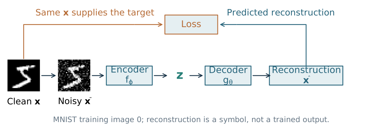
A denoising AE receives corruption but targets the clean image

Copying the corrupted input now disagrees with the clean target.

Four minutes. DAE means denoising autoencoder. Begin with a clean training image, construct a corrupted input, and keep the clean original as the loss target. Examples include randomly masking some input features or adding noise. No externally supplied class label is needed. The corruption is chosen by us and determines what restoration task is learned. The original MNIST image is real; its noisy version is constructed with seed 570, Gaussian noise standard deviation 0.3 and clipping to [0,1]. The reconstruction remains symbolic, not a trained output. A DAE need not have an undercomplete code; the changed objective supplies another constraint. [Sources] source:vincent-denoising-2010, section 3; source:mnist-train-images.

Denoising trains against the original, not the corrupted input

Construct \(\widetilde{\boldsymbol{x}}=c(\boldsymbol{x},\boldsymbol{e})\) using a sampled corruption:

\[\min_{\phi,\theta}\ \mathbb{E}_{\mathbf{x},\mathbf{e}} \left[\frac{1}{d}\left\|\mathbf{x}-g_\theta\!\left(f_\phi\!\left(c(\mathbf{x},\mathbf{e})\right)\right)\right\|_2^2\right].\]

Input sent to encoder	Target used in loss
Corrupted image \(\widetilde{\boldsymbol{x}}\)	Clean image \(\boldsymbol{x}\)

The chosen corruption shapes which structure helps solve the task.

Four minutes. Bold upright x is a random image; italic bold e in the first line denotes a realized corruption draw, while upright bold e in the expectation denotes its random-vector counterpart. The corruption may depend on the clean image; the expectation is over the training image distribution and chosen corruption process. In practice sample images and fresh corruptions for minibatch gradient updates. If the corrupted image is used as the target too, the objective becomes reconstruction of corrupted inputs instead of restoration of the clean original. Zero corruption recovers the vanilla reconstruction objective. Generalization to other corruptions is not automatic. [Sources] source:vincent-denoising-2010, section 3; source:mnist-train-images.

Probability primer

Distributions, expectations, likelihood, and KL

Twenty seconds. Before making the encoder and decoder probabilistic, review the probability tools we will use.

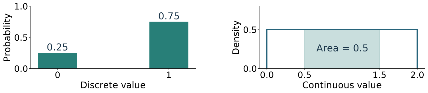
A distribution describes possibilities; a sample is one outcome

For a latent vector, \(\mathbf{z}\sim p\) describes a random draw; \(\boldsymbol{z}\) denotes one realized value.

• Discrete: probabilities at individual values sum to one.
• Continuous: density integrates to one; probability is area over a region, not the height at a point.

Three minutes. Announce a seven-slide probability primer before probabilistic autoencoders. A random variable maps an uncertain outcome to a number; a random vector collects multiple such numbers. A distribution supplies probabilities. Upright bold denotes a random vector; bold italic a realized vector. The plot uses one scalar feature for readability. Discrete values 0 and 1 have probabilities .25 and .75. Uniform density .5 over [0,2] integrates to one; [.5,1.5] has probability .5. For an absolutely continuous variable the probability of one exact value is zero, yet its density can be positive and even exceed one. The same distinction applies in many-dimensional image space. Modeling images continuously is a choice even though stored pixel values are quantized. [Sources] source:goodfellow-probability-2016, sections 3.2–3.3. Adapted in scope from the instructor’s Spring 2026 probability review; examples and plots are original.

Gaussian distributions specify a center and a spread

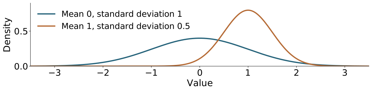
For one feature, \(\textnormal{z}\sim\mathcal{N}(\mu,\sigma^2)\): mean \(\mu\), variance \(\sigma^2\), standard deviation \(\sigma\).

For vectors, \(\mathbf{z}\sim\mathcal{N}(\boldsymbol{\mu},\Sigma)\) uses a covariance matrix.

• Diagonal entries are feature variances; off-diagonal entries are covariances.
• \(\Sigma=I\): independent Gaussian features, each with variance one.

Three minutes. The second Gaussian argument is variance for a scalar and covariance for a vector, never standard deviation. The narrower curve is taller to preserve area one. Covariance records pairwise linear co-variation; diagonal covariance implies independence here because the distribution is jointly Gaussian, not for arbitrary distributions. The standard normal vector also has zero mean. N(mu,diag(sigma²)) lets each feature have its own spread. We need this notation for the probabilistic AE, VAE encoder and diffusion noise, not the full Gaussian normalization or covariance derivations. [Sources] source:goodfellow-probability-2016, sections 3.8 and 3.9.3. Adapted in scope from the instructor’s Spring 2026 probability review; examples and plots are original.

A conditional distribution holds one quantity fixed

\(p(\boldsymbol{x}\mid\boldsymbol{z})\) describes possible images \(\boldsymbol{x}\) for a given code \(\boldsymbol{z}\).

• Fix the code; the distribution over images still integrates to one.
• Changing the code can change the image distribution.
• \(p(\boldsymbol{z}\mid\boldsymbol{x})\) asks a different question: which codes are plausible for a given image?

The joint distribution describes images and codes together:

\[p(\boldsymbol{x},\boldsymbol{z}) =p(\boldsymbol{z})\,p(\boldsymbol{x}\mid\boldsymbol{z}).\]

The vertical bar means given, not division or causation.

Three minutes. Introduce latent code as an internal feature vector, already used by the AE. Read the expression aloud: distribution of x given z. The variables after the bar are held fixed while we vary or integrate the variables before it. For density models p(x|z)=p(x,z)/p(z) where p(z)>0. Conditioning on a value of a continuous variable uses a conditional density; it does not require positive point probability. The product rule itself does not require independence or a causal story. In a later assumed generative model we will choose the factors. p(x|z) and p(z|x) have different domains and are generally different functions. [Sources] source:goodfellow-probability-2016, sections 3.4–3.6. Adapted in scope from the instructor’s Spring 2026 probability review; examples and plots are original.

Marginalization removes a variable; Bayes’ rule reverses conditioning

To describe images without specifying a code, average over possible codes:

\[p(\boldsymbol{x})=\int p(\boldsymbol{x},\boldsymbol{z})\,d\boldsymbol{z} =\int p(\boldsymbol{z})p(\boldsymbol{x}\mid\boldsymbol{z})\,d\boldsymbol{z}.\]

For an observed image, Bayes’ rule gives

\[p(\boldsymbol{z}\mid\boldsymbol{x})= \frac{p(\boldsymbol{x}\mid\boldsymbol{z})\,p(\boldsymbol{z})}{p(\boldsymbol{x})}.\]

• \(p(\boldsymbol{z})\): code distribution before seeing the image (prior).
• \(p(\boldsymbol{z}\mid\boldsymbol{x})\): code distribution after seeing it (posterior).

For discrete codes, replace the integral with a sum.

Three minutes. Marginalization sums or integrates the joint, not the conditional alone. Its product-rule form is a weighted average of conditional image distributions under p(z). Bayes reverses the direction of conditioning and normalizes by p(x), for p(x)>0. This is a relationship among distributions from one joint model, not yet an assertion about how real images are generated. Later the decoder and chosen latent prior define a model and its true posterior. The learned q encoder is an approximation to that posterior, not a replacement for Bayes’ rule. The integral may be hard even when both factors are easy to evaluate. [Sources] source:goodfellow-probability-2016, sections 3.4–3.6 and 3.11. Adapted in scope from the instructor’s Spring 2026 probability review; examples and plots are original.

An expectation is a probability-weighted average

If a loss is \(1\) with probability \(0.75\) and \(5\) with probability \(0.25\), its expectation is \(0.75(1)+0.25(5)=2\).

For a function of a continuous code,

\[\mathbb{E}_{\mathbf{z}\sim q}[h(\mathbf{z})] =\int h(\boldsymbol{z})q(\boldsymbol{z})\,d\boldsymbol{z} \ \approx\ \frac{1}{m}\sum_{j=1}^{m}h(\boldsymbol{z}^{(j)}), \qquad \boldsymbol{z}^{(j)}\text{ sampled from }q.\]

• The integral is the expectation; the sample average estimates it.
• One sample gives a noisy estimate, not the exact average.
• For reconstruction, fix the image and average its loss over codes drawn from its encoder.

Three minutes. A discrete expectation uses a sum weighted by probabilities; the opening arithmetic demonstrates why an unweighted average of the distinct loss values would be wrong. The sample average has equal weights because the samples themselves occur according to q. Use independent draws for the elementary law-of-large-numbers interpretation and assume integrability. More draws generally reduce estimation noise; do not promise monotonic accuracy for each sample batch. VAE training also averages over images, a separate average. h is a placeholder for a scalar function such as loss, not necessarily the identity. Linearity gives E[ah+bg]=aE[h]+bE[g] when finite, but E[g(z)] generally differs from g(E[z]); leave these in notes unless needed. [Sources] source:goodfellow-probability-2016, section 3.8. Adapted in scope from the instructor’s Spring 2026 probability review; examples and plots are original.

Likelihood evaluates an observation we already have

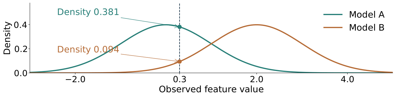
• Sampling: hold the model fixed and draw a new observation.
• Likelihood: hold the observed \(\boldsymbol{x}\) fixed and evaluate \(p_\theta(\boldsymbol{x})\) as the model changes.
• A common loss is \(-\log p_\theta(\boldsymbol{x})\): higher density gives lower loss.

For a decoder, evaluate \(p_\theta(\boldsymbol{x}\mid\boldsymbol{z})\) at the original image.

Three minutes. The illustration compares N(0,1) and N(2,1) at the same scalar observed value .3; all values are analytic, not model results. The scalar picture stands in for an image-density evaluation. A likelihood is the probability mass or density of fixed observed data considered as a function of model parameters, not a probability distribution over parameters. For a continuous model, density at a point is not the probability of that exact point. Negative log density may be negative if density exceeds one; only the ordering matters here. In reconstruction we sample latent codes, then evaluate the original image under the decoder; no new output image draw is needed to compute likelihood. [Sources] source:goodfellow-probability-2016, sections 3.3, 3.13; source:kingma-welling-vae-2013, section 2. Adapted in scope from the instructor’s Spring 2026 probability review; examples and plots are original.

KL compares distributions by averaging a log-density ratio

The Kullback–Leibler divergence is

\[D_{\mathrm{KL}}(q\|p)= \mathbb{E}_{\mathbf{z}\sim q}\!\left[\log\frac{q(\mathbf{z})}{p(\mathbf{z})}\right].\]

• Average under \(q\): disagreement where \(q\) puts weight matters.
• KL is nonnegative and zero when the distributions agree.
• It is directional: generally \(D_{\mathrm{KL}}(q\|p)\ne D_{\mathrm{KL}}(p\|q)\).

For two outcomes, \(q=(0.75,0.25)\) and \(p=(0.5,0.5)\) give \(D_{\mathrm{KL}}(q\|p)\approx0.131\); setting \(p=q\) gives zero.

We will use KL to compare code distributions, including their centers and spreads.

Three minutes. Both densities are evaluated at the same random argument inside the ratio; the expectation is under q. A pointwise log ratio can be negative even though the full average is nonnegative. For the example, .75 log(1.5)+.25 log(.5)=.130812 nats using natural logs. The reverse direction is about .143841, illustrating asymmetry. Zero KL means equality almost everywhere. If p is zero where q has positive mass, KL can be infinite; the Gaussian models used later avoid this support mismatch. KL is not an ordinary symmetric distance. Later distinguish KL to the true posterior in the ELBO gap from the computable KL to the prior in the objective. A point concentrated near zero does not match a Gaussian with unit spread. [Sources] source:goodfellow-probability-2016, section 3.13. Adapted in scope from the instructor’s Spring 2026 probability review; examples and plots are original.