From Probability to Variational Autoencoders

ECE 57000 — November 6, 2026

David I. Inouye

Probability distributions are nonnegative and normalized

	Nonnegative	Total probability is one
Discrete mass	\(p(\boldsymbol{x})\geq0\)	\(\sum_{\boldsymbol{x}}p(\boldsymbol{x})=1\)
Continuous density	\(p(\boldsymbol{x})\geq0\)	\(\int p(\boldsymbol{x})\,d\boldsymbol{x}=1\)

Marginalize: remove \(\boldsymbol{z}\) from a joint distribution by summing or integrating it out.

\[p(\boldsymbol{x})=\sum_{\boldsymbol{z}}p(\boldsymbol{x},\boldsymbol{z}) \quad\text{(discrete codes)},\qquad p(\boldsymbol{x})=\int p(\boldsymbol{x},\boldsymbol{z})\,d\boldsymbol{z} \quad\text{(continuous codes)}.\]

Zero values are allowed. A density can exceed one; its integral must equal one.

Two minutes. November 4 reviewed probability through likelihood and deferred KL. Review validity before marginalization, then conditioning on the next slide. Sums cover the support and integrals the full domain. The joint distribution is over x and z together; marginalizing removes a variable without fixing its value. For continuous densities nonnegativity is understood almost everywhere. [Sources] source:goodfellow-probability-2016, sections3.3–3.4.

Conditioning and Bayes’ rule rearrange the same joint distribution

Conditional distributions (where the denominators are positive):

\[p(\boldsymbol{x}\mid\boldsymbol{z})=\frac{p(\boldsymbol{x},\boldsymbol{z})}{p(\boldsymbol{z})}, \qquad p(\boldsymbol{z}\mid\boldsymbol{x})=\frac{p(\boldsymbol{x},\boldsymbol{z})}{p(\boldsymbol{x})}.\]

Joint decomposition / chain rule:

\[p(\boldsymbol{x},\boldsymbol{z})=p(\boldsymbol{z})p(\boldsymbol{x}\mid\boldsymbol{z}) =p(\boldsymbol{x})p(\boldsymbol{z}\mid\boldsymbol{x}).\]

Bayes’ rule:

\[p(\boldsymbol{z}\mid\boldsymbol{x})= \frac{p(\boldsymbol{x}\mid\boldsymbol{z})p(\boldsymbol{z})}{p(\boldsymbol{x})}.\]

The variables keep their meanings: \(\boldsymbol{x}\) is an image; \(\boldsymbol{z}\) is a code.

Three minutes. Both factorizations describe the same joint and need no independence assumption. The conditioning value is fixed; its positive marginal normalizes the remaining variable. For continuous variables these are density ratios, not ratios of point-event probabilities. The chain rule follows by multiplying either conditional definition by its denominator; equating the two factorizations gives Bayes. Next repeat the deferred KL slide. [Sources] source:goodfellow-probability-2016, sections3.5–3.6 and3.11.

KL compares distributions by averaging a log-density ratio

The Kullback–Leibler divergence is

\[D_{\mathrm{KL}}(q\|p)= \mathbb{E}_{\mathbf{z}\sim q}\!\left[\log\frac{q(\mathbf{z})}{p(\mathbf{z})}\right].\]

Average under \(q\): disagreement where \(q\) puts weight matters.

1. Nonnegative: \(D_{\mathrm{KL}}(q\|p)\geq 0\).
2. Zero when the distributions agree: \(D_{\mathrm{KL}}(q\|q)=\mathbb{E}_{\mathbf{z}\sim q}[\log 1]=0\).

It is directional: generally \(D_{\mathrm{KL}}(q\|p)\ne D_{\mathrm{KL}}(p\|q)\).

For two outcomes, \(q=(0.75,0.25)\) and \(p=(0.5,0.5)\) give \(D_{\mathrm{KL}}(q\|p)\approx0.131\); setting \(p=q\) gives zero.

We will use KL to compare code distributions, including their centers and spreads.

Three minutes. Both densities are evaluated at the same random argument inside the ratio; the expectation is under q. A pointwise log ratio can be negative even though the full average is nonnegative. For the example, .75 log(1.5)+.25 log(.5)=.130812 nats using natural logs. The reverse direction is about .143841, illustrating asymmetry. Zero KL means equality almost everywhere. If p is zero where q has positive mass, KL can be infinite; the Gaussian models used later avoid this support mismatch. KL is not an ordinary symmetric distance. Later distinguish KL to the true posterior in the ELBO gap from the computable KL to the prior in the objective. A point concentrated near zero does not match a Gaussian with unit spread. [Sources] source:goodfellow-probability-2016, section 3.13. Adapted in scope from the instructor’s Spring 2026 probability review; examples and plots are original.

Probabilistic autoencoders

Replace point outputs with distributions

Twenty seconds. Use the probability primer to change both encoder and decoder mappings, then train them to reconstruct the original image.

We can make both encoder and decoder probabilistic

1. Probabilistic AE: replace each point output with a distribution.
2. VAE generative model: add an assumption about where latent codes come from.
3. VAE training: fit the generative model using the encoder to infer codes.

First, encode a point into latent space, then decode back into the same observed space.

Thirty seconds. Follow the instructor’s original progression: probabilistic mappings and their reconstruction objective come before the prior. Denoising changed the input; now change the kind of output produced by each mapping. No prior is assumed in the next examples. [Sources] source:kingma-welling-vae-2013, sections 2–3; source:goodfellow-autoencoders-2016, chapter 14. Adapted from the instructor’s Spring 2026 autoencoder lecture.

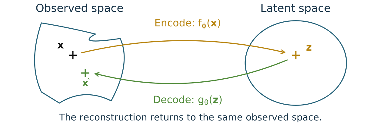
A deterministic AE maps one point to one point

\[\boldsymbol{z}=f_\phi(\boldsymbol{x}),\qquad \widehat{\boldsymbol{x}}=g_\theta(\boldsymbol{z}).\]

Each + is one example or code. The outlines show the spaces where they live.

Two minutes. Reuse the visual grammar of the instructor’s probabilistic-autoencoder drawing: observed space, latent space, individual plus marks, then distributions in later slides. Use one observed space on the left and one latent space on the right. The encoder goes out; the decoder returns to the original space so reconstruction is compared with the original point. Each plus in observed space stands for a whole image, not one pixel. The space boundaries are schematic, not support estimates or learned manifolds. For a fixed input, both deterministic functions produce fixed outputs. [Sources] source:kingma-welling-vae-2013, sections 2–3; source:goodfellow-autoencoders-2016, chapter 14. Adapted from the instructor’s Spring 2026 autoencoder lecture.

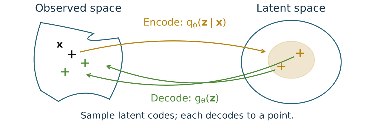
A probabilistic encoder maps an image to a distribution of codes

Replace \(\boldsymbol{z}=f_\phi(\boldsymbol{x})\) with a conditional distribution \(q_\phi(\boldsymbol{z}\mid\boldsymbol{x})\).

The yellow circle is a code distribution; its + marks are sampled codes. The decoder still returns one point per code to the original observed space.

Three minutes. Start with the observed plus on the left. The yellow circle is the encoder’s output distribution, not one large point. Point to each latent plus as a possible sampled code for this same input. The model predicts distribution parameters; a sampling operation produces a code. Shaded regions are schematic probability contours, not hard boundaries: Gaussian samples can lie outside them. At this intermediate stage the decoder is still deterministic: its green plus marks are outputs, not samples from an image distribution. We have not introduced an unconditional latent prior. [Sources] source:kingma-welling-vae-2013, sections 2–3; source:goodfellow-autoencoders-2016, chapter 14. Adapted from the instructor’s Spring 2026 autoencoder lecture.

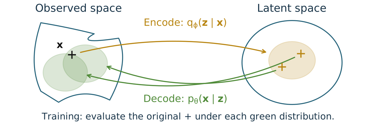
A probabilistic decoder maps each code to a distribution of images

Replace \(\widehat{\boldsymbol{x}}=g_\theta(\boldsymbol{z})\) with \(p_\theta(\boldsymbol{x}\mid\boldsymbol{z})\).

During training, measure the likelihood of the original input image under the distributions represented by the green circles. We sample latent codes, not new images from the decoder.

Four minutes. Follow one latent plus and its green arrow to one green output circle, then the other. A green circle represents the decoder distribution for that code, returning to the same observed space as the original input. There are no green sampled-image marks. Training evaluates the original observed point’s density under each green distribution; it does not draw an image from that distribution. Decoder distribution means need not equal the original input exactly. The original observed plus remains the reconstruction target, not a fresh output draw. This is a conceptual redrawing of the instructor’s circles-and-plus illustration; no model was trained. [Sources] source:kingma-welling-vae-2013, sections 2–3; source:goodfellow-autoencoders-2016, chapter 14. Adapted from the instructor’s Spring 2026 autoencoder lecture.

Gaussian mappings let the networks predict the distribution means

For a first example, hold both covariance matrices fixed at the identity:

\[q_\phi(\boldsymbol{z}\mid\boldsymbol{x}) =\mathcal{N}\!\left(\boldsymbol{z};f_\phi(\boldsymbol{x}),I\right).\]

\[p_\theta(\boldsymbol{x}\mid\boldsymbol{z}) =\mathcal{N}\!\left(\boldsymbol{x};g_\theta(\boldsymbol{z}),I\right).\]

• \(f_\phi\) predicts the center of the latent distribution.
• \(g_\theta\) predicts the center of the image distribution.
• We can also learn the spreads; first keep them fixed to see the mechanism.

Three minutes. This matches the instructor’s original fixed-covariance probabilistic-AE bridge. I has size k by k in the encoder and d by d in the decoder. The neural networks remain deterministic parameter-producing functions; the conditional mappings are probabilistic. Fixed unit observation variance is a simplifying likelihood assumption, not a good default for every normalized image dataset. Diagonal learned encoder covariance comes later. Do not yet call q an approximate posterior of a joint model, because we have not specified the prior. [Sources] source:kingma-welling-vae-2013, sections 2–3; source:goodfellow-autoencoders-2016, chapter 14. Adapted from the instructor’s Spring 2026 autoencoder lecture.

A probabilistic AE can train with expected reconstruction loss

For one observed image, average over sampled codes:

\[\mathcal{J}_{\mathrm{PAE}}(\boldsymbol{x})= \mathbb{E}_{\mathbf{z}\sim q_\phi(\cdot\mid\boldsymbol{x})} [-\log p_\theta(\boldsymbol{x}\mid\mathbf{z})].\]

With the fixed Gaussian mappings, one noise draw gives the estimate

\[\tfrac12\left\|\boldsymbol{x}-g_\theta\!\left(f_\phi(\boldsymbol{x})+ \boldsymbol{\epsilon}\right)\right\|_2^2+C, \qquad \boldsymbol{\epsilon}\sim\mathcal{N}(\boldsymbol{0},I).\]

Evaluate the original \(\boldsymbol{x}\) under the green decoder distribution. Sample codes, not output images.

Four minutes. Follow the original slides’ expected conditional negative-log-likelihood derivation. For unit-covariance Gaussian p, negative log density is half squared error plus d log(2pi)/2. Replace the expectation over codes with z=f(x)+epsilon, then use one sampled epsilon for a Monte Carlo estimate. This is an estimate, not equality to the full expectation. Average this per-image loss over training examples. This is conditional reconstruction likelihood, not the marginal likelihood of a fully specified generative model. No KL term or unconditional latent prior has been added. Connect directly to the returning green circles: evaluate p_theta at the original x for each sampled z. No output image sample is needed to compute this loss. Formal reparameterization gradients come later. [Sources] source:kingma-welling-vae-2013, sections 2–3; source:goodfellow-autoencoders-2016, chapter 14. Adapted from the instructor’s Spring 2026 autoencoder lecture.

Where does the noise enter these two autoencoders?

Both models reconstruct the original clean image.

Which description matches the models we just defined?

A. Denoising AE: noisy input; probabilistic AE: sampled latent code.

B. Denoising AE: sampled latent code; probabilistic AE: noisy input.

C. Both models must use the noisy input as their target.

A. We changed the input for denoising, then changed the mappings for probabilistic autoencoding.

Three minutes including vote and reveal. A is the best answer for the concrete constructions presented. B swaps the location of the noise; C confuses input with target. A probabilistic decoder also defines output randomness, but its likelihood loss evaluates the original target rather than requiring an output draw. The distinctions are pedagogical choices, not mutually exclusive model families: probabilistic encoders can also be used for denoising. This question checks the transition from denoising inputs to probabilistic mappings. [Sources] source:kingma-welling-vae-2013, sections 2–3; source:goodfellow-autoencoders-2016, chapter 14. Adapted from the instructor’s Spring 2026 autoencoder lecture.

VAEs: a generative model

Pair a latent prior with a probabilistic decoder

Twenty seconds. Move from reconstructing an observed image to assumptions that define how to generate a new image.

A prior and decoder define an assumed image-generation process

• We assume a generative process as a way to model images; it need not match how real images are created.
• Pair a probabilistic decoder with a prior on latent codes to define a two-stage sampling process:

1. Sample a latent code: \(\mathbf{z}\sim p(\boldsymbol{z})=\mathcal{N}(\boldsymbol{0},I)\).
2. Sample an image: \(\mathbf{x}\sim p_\theta(\boldsymbol{x}\mid\mathbf{z})\).

\[p_\theta(\boldsymbol{x},\boldsymbol{z}) =p(\boldsymbol{z})\,p_\theta(\boldsymbol{x}\mid\boldsymbol{z}).\]

We will show why an encoder is useful in a few slides.

Three minutes. Emphasize that this is an assumed mathematical image-generation process, not a claim that real images were physically generated by Gaussian latent codes and this decoder. A prior and conditional decoder together define a valid joint model and a two-stage sampling procedure. The prior is the chosen code distribution before observing an image; the standard normal is one convenient assumption, not a distribution automatically discovered by a probabilistic AE. Introduce it only after students understand both conditional mappings and probabilistic reconstruction. The variational encoder and objective complete the VAE construction later; defer the encoder’s usefulness to those slides. Generating a full image draw uses both code randomness and decoder observation randomness; displaying the decoder mean after a prior code draw is another common choice. No encoder is needed to generate. [Sources] source:kingma-welling-vae-2013, sections 2–3; source:goodfellow-autoencoders-2016, chapter 14. Adapted from the instructor’s Spring 2026 autoencoder lecture.

Fitting the generative model means averaging over possible codes

For an observed image, the model assigns density

\[p_\theta(\boldsymbol{x})= \int p(\boldsymbol{z})\,p_\theta(\boldsymbol{x}\mid\boldsymbol{z})\,d\boldsymbol{z}.\]

• We would like to maximize \(\sum_i\log p_\theta(\boldsymbol{x}_i)\).
• The code that produced an observed image is unknown.
• With a nonlinear decoder, this integral is generally difficult to compute exactly.

The encoder helps identify codes that could explain each observed image.

Three minutes. Explain marginalization as combining contributions of different possible latent codes under the prior. Do not imply all codes receive equal weight. Intractability is general for nonlinear neural decoders, not a claim about every latent model. Direct sampling from the prior is possible but can be inefficient for explaining a particular observation. This motivates learned inference and a tractable lower bound, as in the instructor’s old generative-model slide. No derivation of the bound on this slide. [Sources] source:kingma-welling-vae-2013, sections 2–3; source:goodfellow-autoencoders-2016, chapter 14. Adapted from the instructor’s Spring 2026 autoencoder lecture.

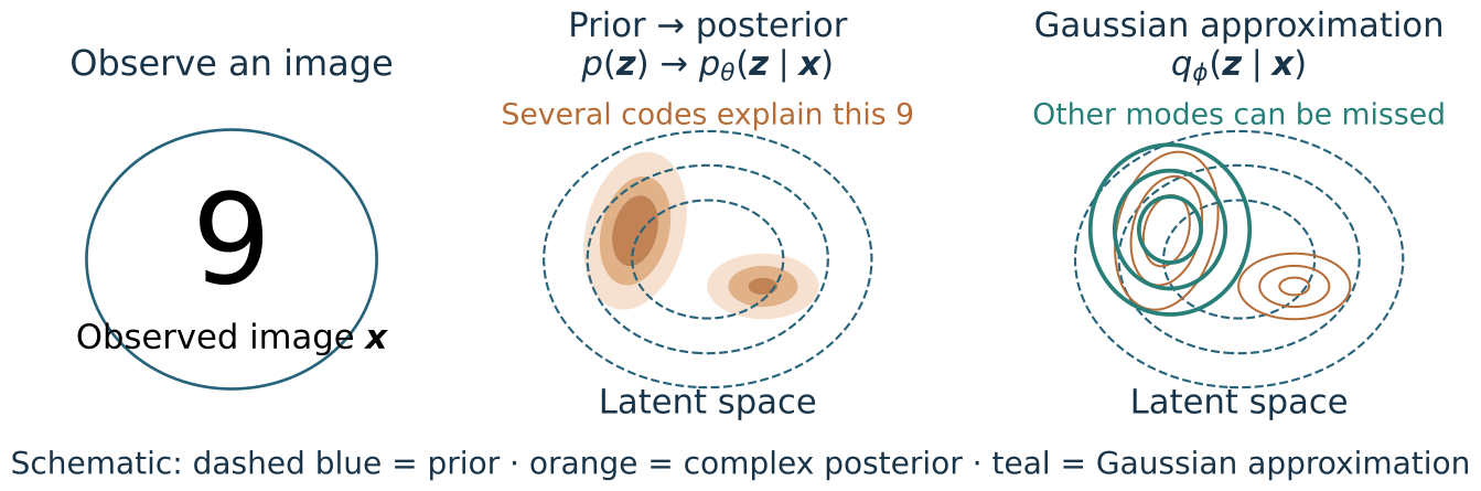
The VAE encoder approximates the codes that explain an image

The prior \(p(\boldsymbol{z})\) is shared; the posterior \(p_\theta(\boldsymbol{z}\mid\boldsymbol{x})\) depends on this image.

\[q_\phi(\boldsymbol{z}\mid\boldsymbol{x})= \mathcal{N}\!\left(\boldsymbol{z};\boldsymbol{\mu}_\phi(\boldsymbol{x}), \operatorname{diag}(\boldsymbol{\sigma}_\phi^2(\boldsymbol{x}))\right) \quad\text{approximates }p_\theta(\boldsymbol{z}\mid\boldsymbol{x}).\]

Four minutes. The figure is an original schematic, not an inferred posterior from the trained demo. Several separated code regions can explain the same image under a nonlinear decoder; a diagonal Gaussian can miss modes and correlations. Conditioning uses the image pixels, not a supplied class label. Connect deterministic and probabilistic AE mappings to the generative model and variational inference role. The exact posterior follows from the prior and decoder by Bayes’ rule but is generally difficult to evaluate because of the marginal likelihood. q is a tractable learned approximation. Mu and positive sigma have k entries; diag squares each standard deviation into a covariance diagonal. q is approximating p_theta(z|x), not the unconditional prior. This distinction explains the ELBO identity in the continuation. The former fixed-I encoder is a restricted special case. [Sources] source:kingma-welling-vae-2013, sections 2–3; source:goodfellow-autoencoders-2016, chapter 14. Adapted from the instructor’s Spring 2026 autoencoder lecture.

Training a VAE

Use the encoder to fit the generative model

Twenty seconds. The encoder approximates the posterior. Now use it to build a tractable objective and compute training gradients.

Encoder samples let us estimate a usable training objective

For a fixed image, draw codes from \(q_\phi(\boldsymbol{z}\mid\boldsymbol{x})\) and define the evidence lower bound (ELBO)

\[\mathcal{L}(\theta,\phi;\boldsymbol{x})= \mathbb{E}_{\mathbf{z}\sim q_\phi(\cdot\mid\boldsymbol{x})} \left[\log p_\theta(\boldsymbol{x},\mathbf{z}) -\log q_\phi(\mathbf{z}\mid\boldsymbol{x})\right].\]

• Evaluate the joint with \(p_\theta(\boldsymbol{x},\boldsymbol{z})=p(\boldsymbol{z})p_\theta(\boldsymbol{x}\mid\boldsymbol{z})\).
• These densities are available; the difficult marginal \(p_\theta(\boldsymbol{x})\) is absent.
• Average sampled values to estimate \(\mathcal{L}\).

Training objective: maximize \(\mathcal{L}\) over $ heta,$ (equivalently, minimize \(-\mathcal{L}\)).

Next, derive why it is a lower bound on image log likelihood.

Three minutes. Introduce the actual quantity before claiming it is computable. The expectation may still require Monte Carlo estimation; tractability means we can evaluate its integrand without the intractable marginal or true posterior. Gaussian KL will later remove sampling from part of this estimate. The next slide explains the lower-bound guarantee. Keep x fixed and average over encoder codes. [Sources] source:kingma-welling-vae-2013, section 2.2, equations 1–3.

Multiplying and dividing by the encoder separates the ELBO and its gap

Fix \(\boldsymbol{x}\); abbreviate \(q=q_\phi(\boldsymbol{z}\mid\boldsymbol{x})\). Every expectation below is under \(q\).

\(\log p_\theta(\boldsymbol{x})\)

\(=\)

\(\mathbb{E}_q[\log p_\theta(\boldsymbol{x})]\)

(fixed image)

\(\,\)

\(=\)

\(\mathbb{E}_q\!\left[\log\frac{p_\theta(\boldsymbol{x},\mathbf{z})}{p_\theta(\mathbf{z}\mid\boldsymbol{x})}\right]\)

(chain rule)

\(\,\)

\(=\)

\(\mathbb{E}_q\!\left[\log\left(\frac{p_\theta(\boldsymbol{x},\mathbf{z})}{q_\phi(\mathbf{z}\mid\boldsymbol{x})}\frac{q_\phi(\mathbf{z}\mid\boldsymbol{x})}{p_\theta(\mathbf{z}\mid\boldsymbol{x})}\right)\right]\)

(multiply by \(q/q\))

\(\,\)

\(=\)

\(\mathbb{E}_q\!\left[\log\frac{p_\theta(\boldsymbol{x},\mathbf{z})}{q_\phi(\mathbf{z}\mid\boldsymbol{x})}\right]+\mathbb{E}_q\!\left[\log\frac{q_\phi(\mathbf{z}\mid\boldsymbol{x})}{p_\theta(\mathbf{z}\mid\boldsymbol{x})}\right]\)

(split the log)

\(\,\)

\(=\)

\({\color{teal}{\mathcal{L}(\theta,\phi;\boldsymbol{x})}}+D_{\mathrm{KL}}\!\left(q_\phi(\cdot\mid\boldsymbol{x})\,\|\,p_\theta(\cdot\mid\boldsymbol{x})\right)\)

(definitions)

Five minutes. Follow the instructor’s Spring 2026 derivation: put the fixed log evidence inside an expectation, use the posterior factorization, multiply and divide by q, then split the logarithm into two expectations. The first is exactly the previously defined ELBO; the second is the KL to the true posterior. Assume positive densities on the support and finite expectations, as in the Gaussian examples. Keep the first equality visible; reveal one justified row at a time. [Sources] source:kingma-welling-vae-2013, section2.2, equations1–3. Adapted from lectures/ece473-spring-2026/14-autoencoders.qmd, Derivation of VAE Objective.

The ELBO gives a lower bound on image log likelihood

For one image, the following identity connects inference and generation:

\[\log p_\theta(\boldsymbol{x})= \underbrace{\mathcal{L}(\theta,\phi;\boldsymbol{x})}_{\text{ELBO}} +\underbrace{D_{\mathrm{KL}}\!\left(q_\phi(\cdot\mid\boldsymbol{x})\,\|\, p_\theta(\cdot\mid\boldsymbol{x})\right)}_{\text{gap from approximate inference}}.\]

Because KL is nonnegative, \(\mathcal{L}(\theta,\phi;\boldsymbol{x})\leq\log p_\theta(\boldsymbol{x})\).

• Fit \(\theta\) and \(\phi\) by maximizing this evidence lower bound.
• The bound is tight when the encoder equals the true posterior.

Two minutes. Read the conclusion of the preceding revealed derivation. Define L=E_q[log p_theta(x,z)-log q(z|x)]. Substitute p_theta(x,z)=p_theta(z|x)p_theta(x), separate the expectation, and rearrange to obtain the displayed identity. This KL compares the encoder with the true posterior, not with the prior. The next slide rewrites the same ELBO using the joint factorization to obtain a different, tractable KL against the prior. Joint optimization need not monotonically tighten the gap because theta changes the true posterior. [Sources] source:kingma-welling-vae-2013, sections 2–3; source:goodfellow-autoencoders-2016, chapter 14. Adapted from the instructor’s Spring 2026 autoencoder lecture.