Variational Autoencoders (continued)

ECE 57000 — November 9, 2026

David I. Inouye

The encoder helps us fit a latent generative model

• Generate: sample a code from the prior, then an image from the decoder.
• Infer: given an image, the encoder approximates its posterior over codes.
• Train: maximize an ELBO that we can estimate without the difficult image marginal.

\[p_\theta(\boldsymbol{x},\boldsymbol{z})=p(\boldsymbol{z})p_\theta(\boldsymbol{x}\mid\boldsymbol{z}), \qquad q_\phi(\boldsymbol{z}\mid\boldsymbol{x})\approx p_\theta(\boldsymbol{z}\mid\boldsymbol{x}).\]

Today: turn the bound into a loss, compute gradients, then inspect what the trained model can do.

Three minutes. November 6 developed probabilistic mappings, the assumed latent generative process, approximate inference and the ELBO derivation. Recall the distinct roles of the fixed prior, learned decoder and image-specific encoder. The encoder is needed for this training method, not for prior-based generation. Next repeat the exact final lower-bound slide; do not repeat the entire derivation. The recorded handwritten graph illustrated the bound, not guaranteed monotonic improvement of the exact likelihood. [Sources] source:kingma-welling-vae-2013, sections2–3.

The ELBO gives a lower bound on image log likelihood

For one image, the following identity connects inference and generation:

\[\log p_\theta(\boldsymbol{x})= \underbrace{\mathcal{L}(\theta,\phi;\boldsymbol{x})}_{\text{ELBO}} +\underbrace{D_{\mathrm{KL}}\!\left(q_\phi(\cdot\mid\boldsymbol{x})\,\|\, p_\theta(\cdot\mid\boldsymbol{x})\right)}_{\text{gap from approximate inference}}.\]

Because KL is nonnegative, \(\mathcal{L}(\theta,\phi;\boldsymbol{x})\leq\log p_\theta(\boldsymbol{x})\).

• Fit \(\theta\) and \(\phi\) by maximizing this evidence lower bound.
• The bound is tight when the encoder equals the true posterior.

Two minutes. Read the conclusion of the preceding revealed derivation. Define L=E_q[log p_theta(x,z)-log q(z|x)]. Substitute p_theta(x,z)=p_theta(z|x)p_theta(x), separate the expectation, and rearrange to obtain the displayed identity. This KL compares the encoder with the true posterior, not with the prior. The next slide rewrites the same ELBO using the joint factorization to obtain a different, tractable KL against the prior. Joint optimization need not monotonically tighten the gap because theta changes the true posterior. [Sources] source:kingma-welling-vae-2013, sections 2–3; source:goodfellow-autoencoders-2016, chapter 14. Adapted from the instructor’s Spring 2026 autoencoder lecture.

The VAE loss balances reconstruction and agreement with the prior

Factor \(p_\theta(\boldsymbol{x},\boldsymbol{z})=p(\boldsymbol{z})p_\theta(\boldsymbol{x}\mid\boldsymbol{z})\) inside the ELBO:

\[\mathcal{L}=\mathbb{E}_q[\log p_\theta(\boldsymbol{x}\mid\mathbf{z})] +\mathbb{E}_q\!\left[\log\frac{p(\mathbf{z})}{q_\phi(\mathbf{z}\mid\boldsymbol{x})}\right].\]

Minimize the negative ELBO:

\[\mathcal{J}=-\mathcal{L}= \underbrace{\mathbb{E}_q[-\log p_\theta(\boldsymbol{x}\mid\mathbf{z})]}_{\text{reconstruction penalty}} +\underbrace{D_{\mathrm{KL}}\!\left(q_\phi(\cdot\mid\boldsymbol{x})\,\|\,p(\cdot)\right)}_{\text{prior regularization}}.\]

Two different KL terms	Meaning
\(D_{\mathrm{KL}}(q_\phi(\cdot\mid\boldsymbol{x})\|p_\theta(\cdot\mid\boldsymbol{x}))\)	True posterior: inference error for this image
\(D_{\mathrm{KL}}(q_\phi(\cdot\mid\boldsymbol{x})\|p(\cdot))\)	Prior: regularization toward shared sampling codes

Five minutes. Define negative log likelihood as a penalty for assigning low probability density to the observed image. The expectation averages over codes from this image’s encoder distribution, not over prior samples. The ELBO identity just introduced compares q with the true posterior. Factoring p_theta(x,z)=p(z)p_theta(x|z) instead rewrites negative ELBO as reconstruction plus KL to the prior. These two KL terms are different. Both theta and phi are learned; in this example p is fixed. This is the negative evidence lower bound, or negative ELBO. Minimizing it maximizes a lower bound on log p_theta(x); do not claim it is exactly maximum likelihood or that the approximate posterior must equal the prior. The preceding identity motivates the bound; its factorization gives this computable form. For continuous densities negative log likelihood need not be nonnegative, though its optimization role is unchanged. [Sources] source:kingma-welling-vae-2013, sections 2–3 and appendix B.

\(\beta\) controls how strongly codes must agree with the prior

\[\mathcal{J}_\beta= \underbrace{\mathbb{E}_q[-\log p_\theta(\boldsymbol{x}\mid\mathbf{z})]}_{\text{reconstruction}} +\beta\,\underbrace{D_{\mathrm{KL}}(q_\phi(\cdot\mid\boldsymbol{x})\|p(\cdot))}_{\text{prior regularization}}.\]

Weight	What we optimize
\(\beta=0\)	Probabilistic autoencoder: reconstruction alone
\(0<\beta<1\)	Weaker prior regularization
\(\beta=1\)	Standard VAE: exactly the negative ELBO
\(\beta>1\)	Stronger prior regularization (β-VAE)

More prior pressure can reduce information about the image and worsen reconstruction.

Side point: as \(\beta\to\infty\), \(q_\phi(\boldsymbol{z}\mid\boldsymbol{x})=p(\boldsymbol{z})\) gives zero KL. A sufficiently expressive decoder could still fit images with \(p_\theta(\boldsymbol{x}\mid\boldsymbol{z})=p_\theta(\boldsymbol{x})\), although \(\mathbf{x}\) and \(\mathbf{z}\) are independent.

Four minutes. Beta is the conventional name for this weighting, verified against Higgins et al. section2 equation4. Hold reconstruction scaling fixed when comparing beta. At beta0 this is the earlier probabilistic AE, with no constraint making prior samples useful. For beta other than1 this is not the ordinary negative ELBO; for beta>=1 its negative remains a possibly looser lower bound because the additional KL penalty is nonnegative, whereas beta<1 has no general lower-bound guarantee. Increased beta may encourage simpler representations but does not guarantee disentanglement. Side point only: with KL zero feasible and reconstruction bounded below, increasing beta strongly favors q=p. A sufficiently expressive decoder could still model data with p_theta(x|z)=p_theta(x), making x and z independent and the true posterior equal to the prior. Then integrating out z recovers p_theta(x); good marginal generation need not require useful codes. A fixed-variance Gaussian decoder independent of z is only one Gaussian, so cannot generally fit a multimodal image distribution. Do not claim finite beta always collapses or a simple decoder can reproduce arbitrary data. [Sources] source:higgins-beta-vae-2017, section2 equation4; source:kingma-welling-vae-2013, section2. The independence example is an explicit mathematical consequence, not an experimental claim.

A Gaussian decoder turns likelihood into scaled squared error

Part 1 of the VAE objective: reconstruction.

Let the decoder predict an image mean \(g_\theta(\boldsymbol{z})\) with fixed variance \(\tau^2\):

\[p_\theta(\boldsymbol{x}\mid\boldsymbol{z}) =\mathcal{N}\!\left(\boldsymbol{x};g_\theta(\boldsymbol{z}),\tau^2 I\right).\]

Then, for a \(d\)-feature image,

\[-\log p_\theta(\boldsymbol{x}\mid\boldsymbol{z}) =\frac{\|\boldsymbol{x}-g_\theta(\boldsymbol{z})\|_2^2}{2\tau^2} +\frac{d}{2}\log(2\pi\tau^2).\]

• \(\tau\) is the decoder observation spread; \(\boldsymbol{\sigma}\) describes encoder codes.
• With fixed \(\tau\), the last term is constant during training.
• Changing the error scale changes its balance with KL.

Three minutes. Reconnect the earlier unit-covariance probabilistic-AE example to the VAE reconstruction term. The norm sums squared errors over features; dividing that sum by d without also rescaling KL changes the objective. Tau is fixed here, so dropping the constant does not change optimization; if tau is learned, the log-variance term must remain. A Gaussian likelihood is an explicit observation-model choice, not a requirement for all VAEs. [Sources] source:kingma-welling-vae-2013, appendix C.2.

For Gaussian codes, we can calculate KL directly

Part 2 of the VAE objective: regularization. Compare the encoder’s approximate posterior with the prior:

\[q_\phi(\cdot\mid\boldsymbol{x})=\mathcal{N}\!\left(\boldsymbol{\mu}_\phi(\boldsymbol{x}), \operatorname{diag}(\boldsymbol{\sigma}_\phi^2(\boldsymbol{x}))\right), \qquad p(\cdot)=\mathcal{N}(\boldsymbol{0},I).\]

\[D_{\mathrm{KL}}\!\left(q_\phi(\cdot\mid\boldsymbol{x})\,\|\,p(\cdot)\right) =\frac{1}{2}\sum_{j=1}^{k}\left(\mu_j^2+\sigma_j^2-1-\log\sigma_j^2\right).\]

Here \(\boldsymbol{\mu}=\boldsymbol{\mu}_\phi(\boldsymbol{x})\) and \(\boldsymbol{\sigma}=\boldsymbol{\sigma}_\phi(\boldsymbol{x})\) are this image’s encoder outputs.

• Mean \(\boldsymbol{0}\) and spread \(\boldsymbol{1}\) match the prior and give zero KL.
• This term is analytic: no latent-code sampling is needed.

Three minutes. Suppress phi and x in mu and sigma only for readability; these remain encoder outputs for the current image. The sum is over k latent features, not d pixels. Natural logs give units of nats. Both extremely small and extremely large standard deviations cost KL. This is the negative of the sign convention used for the KL contribution to the maximized ELBO in appendix B; our minimized objective has positive KL. [Sources] source:kingma-welling-vae-2013, sections 2–3 and appendix B.

The encoder changes the distribution inside the expectation

To maximize the ELBO, we need \(\nabla_{\theta,\phi}\mathcal{L}\) (or minimize \(\mathcal{J}=-\mathcal{L}\)). The Gaussian KL is explicit; reconstruction still needs an expectation.

Let \(\ell_\theta(\boldsymbol{z})=-\log p_\theta(\boldsymbol{x}\mid\boldsymbol{z})\) for fixed \(\boldsymbol{x}\):

\[\nabla_\phi\mathbb{E}_{\mathbf{z}\sim q_\phi}[\ell_\theta(\mathbf{z})] =\nabla_\phi\int q_\phi(\boldsymbol{z}\mid\boldsymbol{x})\ell_\theta(\boldsymbol{z})\,d\boldsymbol{z} \ne \mathbb{E}_{q_\phi}[\nabla_\phi\ell_\theta(\mathbf{z})]\quad\text{in general}.\]

• At a fixed code, \(\ell_\theta\) has no direct \(\phi\) dependence; the naive right side is zero.
• But changing the encoder changes which codes are likely.
• We need to move \(\phi\) into a differentiable function of parameter-independent noise.

Four minutes. The issue is not that differentiating an integral is forbidden. Under regularity one can differentiate q times the integrand; the missing derivative of q is precisely the problem with naively moving the gradient into an expectation and holding the sampled z fixed. Score-function estimators are another option, but not today’s method. Theta has an ordinary gradient inside the expectation here because q depends on phi, not theta. [Sources] source:kingma-welling-vae-2013, section2.3.

Reparameterization makes sampling a differentiable calculation

For a diagonal Gaussian encoder, an exact alternative sampling procedure is

\[\boldsymbol{\epsilon}\sim\mathcal{N}(\boldsymbol{0},I),\qquad \boldsymbol{z}=\boldsymbol{\mu}_\phi(\boldsymbol{x})+ \boldsymbol{\sigma}_\phi(\boldsymbol{x})\odot\boldsymbol{\epsilon}.\]

1. Draw noise from a distribution independent of the encoder parameters.
2. Scale it by the encoder’s standard deviations.
3. Shift it by the encoder’s means.

The transformed code has exactly distribution \(q_\phi(\boldsymbol{z}\mid\boldsymbol{x})\):

\[\nabla_\phi\mathbb{E}_{q_\phi}[\ell_\theta(\mathbf{z})] =\mathbb{E}_{\boldsymbol{\epsilon}\sim\mathcal{N}(\boldsymbol{0},I)} \!\left[\nabla_\phi\ell_\theta\!\left(\boldsymbol{\mu}_\phi+\boldsymbol{\sigma}_\phi\odot\boldsymbol{\epsilon}\right)\right].\]

Now the noise distribution is fixed. More complex reparameterizations exist; this Gaussian case is the simplest common one.

Three minutes. The gradient identity holds under the usual differentiability and integrability conditions; x is suppressed in mu and sigma. Epsilon here denotes the realized draw after sampling; the formula specifies a sampling procedure. Elementwise multiplication is denoted odot. The resulting z has exactly the diagonal Gaussian distribution q_phi(z|x); this is not a new approximate distribution. Differentiation holds the sampled epsilon fixed for this update, not forever across training. This pathwise gradient avoids differentiating a black-box sampling instruction and supplies reconstruction gradients to phi. KL is already differentiable analytically. [Sources] source:kingma-welling-vae-2013, sections 2–3 and appendix B.

Fixed noise lets backpropagation follow the encoder-to-loss path

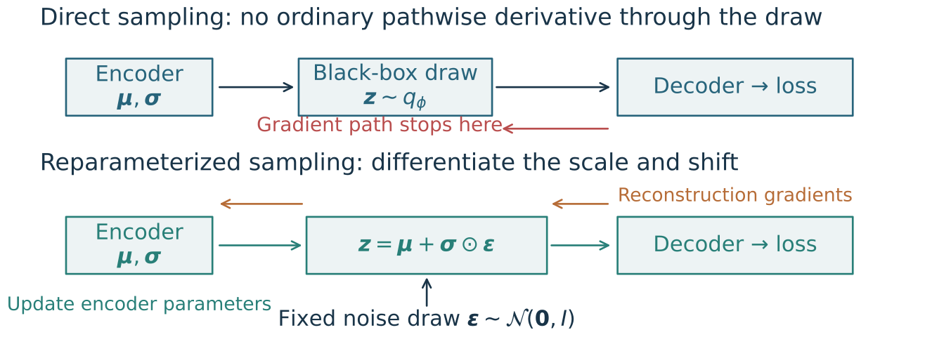
Hold \(\boldsymbol{\epsilon}\) fixed for this gradient calculation; differentiate the scale and shift, not the random draw.

Three minutes. Orange arrows show reconstruction gradients moving right to left. The decoder gradient works in both diagrams; the encoder reconstruction gradient needs the pathwise transformation in the bottom diagram. A black-box random draw is not an ordinary deterministic differentiable operator; this does not rule out score-function estimators. Once the noise is an input, partial z_j/partial mu_j=1 and partial z_j/partial sigma_j=epsilon_j. The analytic KL adds another encoder gradient path. Resample noise on the next update. [Sources] source:kingma-welling-vae-2013, section2.3. Original computational-graph illustration.

Monte Carlo sampling estimates the expectation and its gradient

Draw \(M\) independent noises and form codes via the reparameterization trick:

\[\boldsymbol{\epsilon}^{(m)}\sim\mathcal{N}(\boldsymbol{0},I),\qquad \boldsymbol{z}^{(m)}=\boldsymbol{\mu}_\phi(\boldsymbol{x})+ \boldsymbol{\sigma}_\phi(\boldsymbol{x})\odot\boldsymbol{\epsilon}^{(m)}.\]

\[\widehat{\mathcal{J}}_\beta= \underbrace{\frac{1}{M}\sum_{m=1}^{M}-\log p_\theta(\boldsymbol{x}\mid\boldsymbol{z}^{(m)})}_{\text{Monte Carlo reconstruction estimate}} +\beta\,\underbrace{D_{\mathrm{KL}}(q_\phi(\cdot\mid\boldsymbol{x})\|p(\cdot))}_{\text{closed-form Gaussian KL}}.\]

• Backpropagate \(\nabla_{\theta,\phi}\widehat{\mathcal{J}}_\beta\); at \(\beta=1\), it estimates \(-\nabla_{\theta,\phi}\mathcal{L}\).
• Usually \(M=1\) per image; average over a minibatch and draw fresh noise each update.
• Reparameterization supplies the gradient path; Monte Carlo approximates the integral.

Four minutes. The estimator and its pathwise gradient are unbiased for the corresponding fixed-image objective under the usual interchange conditions; a single draw has variance and need not equal the expectation. Averaging across images also estimates the dataset objective. Gaussian KL is evaluated exactly from encoder parameters, not estimated using that single code. The VAE paper reports L=1 with sufficiently large minibatches; use M here to avoid confusing sample count with calligraphic L for ELBO. [Sources] source:kingma-welling-vae-2013, section2.3, equations6–7 and algorithm1.

Each minibatch trains the encoder and decoder together

For a batch \(\{\boldsymbol{x}_i\}_{i=1}^{B}\), compute all \(B\) examples in parallel:

Step	Batched computation (each \(i=1,\ldots,B\))
1. Encode	\((\boldsymbol{\mu}_i,\boldsymbol{s}_i)=f_\phi(\boldsymbol{x}_i)\); \(\boldsymbol{s}_i\) is log variance
2. Sample codes	\(\boldsymbol{\epsilon}_i\sim\mathcal{N}(\boldsymbol{0},I)\); \(\boldsymbol{z}_i=\boldsymbol{\mu}_i+\exp(\boldsymbol{s}_i/2)\odot\boldsymbol{\epsilon}_i\)
3. Decode and score	\(r_i=-\log p_\theta(\boldsymbol{x}_i\mid\boldsymbol{z}_i)\); \(k_i=\tfrac12\sum_j(\mu_{ij}^2+e^{s_{ij}}-1-s_{ij})\)
4. Average the loss	\(\widehat{\mathcal{J}}_\beta=\tfrac1B\sum_{i=1}^{B}(r_i+\beta k_i)\)
5. Update both networks	\(\theta\leftarrow\theta-\eta\nabla_\theta\widehat{\mathcal{J}}_\beta\); \(\phi\leftarrow\phi-\eta\nabla_\phi\widehat{\mathcal{J}}_\beta\)

One fresh code per image. At \(\beta=1\), the batch loss estimates the average negative ELBO.

Five minutes. The equations use per-image vectors while the implementation stacks their transposes into matrices: X has shape[B,d]; means, log variances, epsilon and Z have shape[B,k]. Both encoder and decoder run on the whole batch. Draw independent noise for every image and latent feature. The decoder computes the conditional distribution parameters for each Z row; r_i evaluates the original X row under that distribution. For the preceding fixed-Gaussian likelihood, r_i is summed squared error divided by2tau^2 plus its constant; for the later Bernoulli demo it is summed binary cross entropy. Sum KL over latent features j and reconstruction over image features, then average over batch index i. Never average over latent features in one term while silently changing the relative scale of the other. Exp and multiplication act elementwise. Backpropagate once through the averaged loss, keeping the sampled epsilon fixed for this gradient, and then update both parameter sets using gradients from the same forward pass. The displayed updates are plain SGD for clarity; Adam can use these same gradients. With beta1 and one code per image this is the minibatch Monte Carlo estimate of negative ELBO. [Sources] source:kingma-welling-vae-2013, algorithm1 and appendixB.

What happens if we train using only the KL term?

The prior is \(\mathcal{N}(\boldsymbol{0},I)\) and the encoder can represent it exactly.

Which encoder minimizes KL for every image?

A. A different narrow distribution for each image.

B. A point concentrated at zero for every image.

C. The same standard Gaussian for every image.

C. Matching both center and spread gives zero KL; that encoder distribution carries no image-specific information.

Three minutes including vote and reveal. A favors identifying individual images, but that is not the KL-only goal. B matches the mean but not the spread; Gaussian KL grows without bound as variance approaches zero. The full objective adds reconstruction, which rewards informative codes. KL-only training does not train the decoder; no image-quality conclusion follows. Do not claim the full VAE necessarily collapses. This second question tests why the objective needs both terms. [Sources] source:kingma-welling-vae-2013, section2.2 and appendixB.

After training, the encoder provides representations and reconstructions

• Represent: \(\boldsymbol{x}\mapsto\boldsymbol{\mu}_\phi(\boldsymbol{x})\) gives a feature vector for downstream tasks.
• Reconstruct: encode an image, then decode its mean code (or a sampled code).

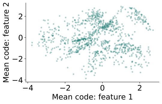
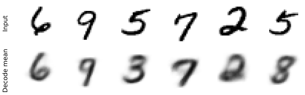
Selected held-out MNIST examples; this demo uses a Bernoulli decoder. Reconstructions can lose detail.

Three minutes. The encoder is useful after training even though generation itself only needs the decoder. Mu is a convenient deterministic representation; sigma also describes uncertainty in the approximate posterior. Code usefulness requires downstream evaluation. Real reproducible demo, not invented outputs: scripts/vae_usage_demo.py and images/07-02-variational-autoencoders/usage-demo.json. Seed570; MNIST archived training images0:12000 used for fitting,59000:60000 held out internally; 40epochs, two latent features, beta1, Bernoulli observation model. Selected held-out offsets[0,6,2,3,4,5]. Instructor requested replacing offset1, whose3 reconstructs ambiguously as8, with offset6 for mechanism clarity; these selected illustrations are not a quality estimate. Display decoder means. This demo uses a Bernoulli decoder; the earlier Gaussian likelihood was an algebra example. [Sources] source:mnist-train-images; source:kingma-welling-vae-2013, sections3 and5.

Interpolation uses encoded endpoints; generation needs only the decoder

Interpolate: encode two images, then decode \(\boldsymbol{z}(a)=(1-a)\boldsymbol{\mu}_1+a\boldsymbol{\mu}_2\).

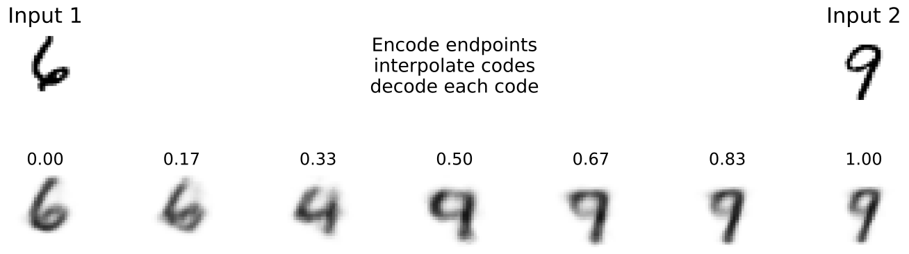
Generate: draw \(\boldsymbol{z}\sim p(\boldsymbol{z})\) and decode; no input image or encoder is needed.

Decoder means shown; smooth interpolation does not guarantee good prior samples.

Three minutes. Same reproducible model as the preceding slide. Selected internally held-out offsets[0,6] provide the interpolation endpoints, with seven equally spaced weights; offset1 was replaced at instructor request as on the preceding slide. These are selected illustrations, not representative-quality evidence; generation uses the first eight standard-normal codes with seed571, without selection. A full image sample also draws from the decoder’s Bernoulli likelihood; plotting its mean makes the model’s expected pixels readable. Interpolation codes are not generally prior draws. Show imperfect samples as well as recognizable ones; this small two-feature model is not a benchmark. [Sources] source:mnist-train-images; source:kingma-welling-vae-2013, sections3 and5.

A trained VAE still needs evidence for its intended use

Intended use	Evidence to inspect
Reconstruct an observed image	Held-out reconstruction under the stated loss
Generate new images	Fresh prior samples: quality, diversity and failure cases
Use the learned code for another task	Held-out performance on that downstream task

Audit the assumptions: chosen prior, decoder likelihood and approximate-posterior family.

A good training objective gives a learning procedure; it does not guarantee all three uses succeed.

Three minutes. Close the VAE story before moving to diffusion. These are separate evaluations, not interchangeable demonstrations. A diagonal Gaussian encoder can limit posterior approximation, and the chosen likelihood/prior may be a poor fit; optimization and finite data are additional limitations. No new measured results are claimed. This is a concise local audit; the full value-driven evaluation unit still follows diffusion. [Sources] source:kingma-welling-vae-2013, sections2 and5; source:goodfellow-autoencoders-2016, chapter14.

Diffusion returns to denoising at many noise levels

Two ways to generate an image:

1. VAE: sample a latent code, then decode an image.
2. Diffusion: start from noise and form an image through repeated denoising steps.

The next model learns how to denoise at different noise levels, using the noise level as an input.

Remember the denoising AE: corrupted input, clean-image information as the training signal.

Two minutes. This is the next-topic bridge, not the full diffusion lesson. In standard DDPM the network predicts the added noise at a sampled noise level; a clean training image is used to construct the pair. Sampling uses predictions in a specified reverse process, not simply repeated applications of an arbitrary DAE. Restore the deferred ambiguity point here later: at high noise many clean originals are plausible, motivating a generative process rather than claiming recovery of one known original. Standard reverse steps are sequential. [Sources] source:ho-ddpm-2020, sections 2–3. [Sources] source:kingma-welling-vae-2013, sections 2–3 and appendix B.

Generating images by diffusion

David I. Inouye

Dynamic Content · Last Updated: November 9, 2026

Arc 7 · Image generation and evaluation

Denoising → the circle example → many noise levels → reverse generation

Thirty seconds. Start with the familiar denoising task, remove the architectural restriction, and change the prediction target. The circle example then motivates multiple noise levels before introducing an additive Gaussian walk. This teaching parameterization follows the earlier course slides; it is not the variance-preserving DDPM schedule. [Sources] source:goodfellow-autoencoders-2016, section14.5; source:ho-ddpm-2020, sections2–3 for the general forward/reverse framework.

A denoising autoencoder predicts the clean input

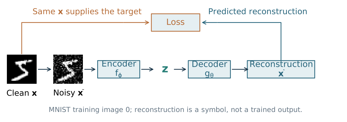
\[\boldsymbol{y}=\boldsymbol{x}+\sigma\boldsymbol{\epsilon},\qquad \boldsymbol{\epsilon}\sim\mathcal N(\boldsymbol 0,I),\qquad \widehat{\boldsymbol{x}}=g_\theta(f_\phi(\boldsymbol{y})).\]

Input: corrupted image. Target: original clean image.

Two minutes. Recall the DAE diagram already taught. For this continuation choose additive Gaussian corruption with fixed sigma>0 and squared-error reconstruction. The encoder/decoder architecture is one way to implement the predictor. Original diagram reused from the AE topic. [Sources] source:goodfellow-autoencoders-2016, section14.5.

Denoising needs a predictor, not a required bottleneck

\[\widehat{\boldsymbol{x}}=D_\theta(\boldsymbol{y}),\qquad \min_\theta\;\mathbb E\!\left[\|\boldsymbol{x}-D_\theta(\boldsymbol{x}+\sigma\boldsymbol{\epsilon})\|^2\right].\]

• Directly map a noisy image to a clean-image prediction of the same shape.
• We can use any suitable neural network; an explicit latent code is optional.
• An encoder–decoder or U-Net can still be a useful architecture.

Two minutes. Separate the statistical task from the architecture. We no longer require a separately interpreted code or a compression bottleneck; this does not prohibit downsampling and upsampling inside a U-Net. Both expectations average over clean training data and independent standard Gaussian noise. [Sources] source:goodfellow-autoencoders-2016, section14.5; source:ho-ddpm-2020, section3.3.

Predicting the clean image and predicting its noise are equivalent

For \(\boldsymbol{y}=\boldsymbol{x}+\sigma\boldsymbol{\epsilon}\) at a fixed \(\sigma>0\):

\[\widehat{\boldsymbol{x}}=\boldsymbol{y}-\sigma\epsilon_\theta(\boldsymbol{y}), \qquad \widehat{\boldsymbol{\epsilon}}=\frac{\boldsymbol{y}-D_\theta(\boldsymbol{y})}{\sigma}.\]

The squared errors differ by a constant:

\[\|\boldsymbol{x}-\widehat{\boldsymbol{x}}\|^2 =\sigma^2\|\boldsymbol{\epsilon}-\widehat{\boldsymbol{\epsilon}}\|^2.\]

Same prediction problem; a different output parameterization.

Three minutes. Define epsilon_theta as predicting standard noise, not sigma times noise. For any clean predictor the residual gives a noise predictor and conversely. With compatible function classes the fixed-sigma population optima correspond. This does not promise identical optimization trajectories for separately parameterized networks. Across varying sigma the factor changes: unweighted clean MSE and unweighted noise MSE weight levels differently. Show that algebra before changing the objective. Original derivation from the stated corruption equation; compare the noise parameterization in source:ho-ddpm-2020, section3.2.