Generating Images by Diffusion (continued)

ECE 57000 — November 11, 2026

David I. Inouye

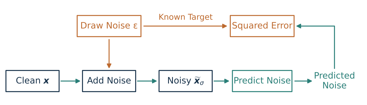
Known corruption lets us learn a denoising task

• November 9 completed VAE training: reconstruction and prior regularization train both networks.
• Diffusion returns to denoising: predict a clean image from its corrupted version.
• At fixed noise scale, predicting the clean image or its added noise gives equivalent targets.

Today: learn noisy scores, connect several noise levels, then view generation as solving an SDE or ODE.

Three minutes. Recall the distinction between generating new images and reconstructing an observed one. November 9 finished at the clean/noise equivalence slide, which follows with the instructor-requested tilde notation. The trained circle example distinguishes score estimation error from the noisy target itself. The instructor confirmed November 11 for this continuation. [Sources] source:goodfellow-autoencoders-2016, section14.5; source:ho-ddpm-2020, sections2–3.

Predicting the clean image and predicting its noise are equivalent

For \(\widetilde{\boldsymbol{x}}_\sigma=\boldsymbol{x}+\sigma\boldsymbol{\epsilon}\) at a fixed \(\sigma>0\):

\[\widehat{\boldsymbol{x}}=\widetilde{\boldsymbol{x}}_\sigma-\sigma\epsilon_{\theta,\sigma}(\widetilde{\boldsymbol{x}}_\sigma), \qquad \widehat{\boldsymbol{\epsilon}}=\frac{\widetilde{\boldsymbol{x}}_\sigma-D_{\theta,\sigma}(\widetilde{\boldsymbol{x}}_\sigma)}{\sigma}.\]

The squared errors differ by a constant:

\[\|\boldsymbol{x}-\widehat{\boldsymbol{x}}\|^2 =\sigma^2\|\boldsymbol{\epsilon}-\widehat{\boldsymbol{\epsilon}}\|^2.\]

Same prediction problem; a different output parameterization.

Three minutes. Define epsilon_theta as predicting standard noise, not sigma times noise. For any clean predictor the residual gives a noise predictor and conversely. With compatible function classes the fixed-sigma population optima correspond. This does not promise identical optimization trajectories for separately parameterized networks. Across varying sigma the factor changes: unweighted clean MSE and unweighted noise MSE weight levels differently. Show that algebra before changing the objective. Original derivation from the stated corruption equation; compare the noise parameterization in source:ho-ddpm-2020, section3.2.

The noise we draw becomes a supervised target

\[J(\theta)=\mathbb E_{\mathbf{x},\boldsymbol{\epsilon}} \left[\|\boldsymbol{\epsilon}-\epsilon_{\theta,\sigma}(\boldsymbol{x}+\sigma\boldsymbol{\epsilon})\|^2\right].\]

No noise labels need to be collected: we constructed the corruption.

Two minutes. Sigma is still one fixed positive noise level. Expectation notation denotes draws from the clean-data distribution and independent standard Gaussian noise; bold italic epsilon is the sampled realization inside the computation. The network sees only the corrupted input, while the known noise goes to the loss. It generally cannot recover the exact realized noise for every ambiguous input. [Sources] source:ho-ddpm-2020, section3.2, for noise prediction; this fixed-noise version is an original specialization.

One minibatch update learns noise prediction at one level

Fix \(\sigma>0\). For each batch of \(B\) clean images:

Step	Computation, \(i=1,\ldots,B\)
Draw noise	\(\boldsymbol{\epsilon}_i\sim\mathcal N(\boldsymbol 0,I)\) independently
Corrupt	\(\widetilde{\boldsymbol{x}}_{\sigma,i}=\boldsymbol{x}_i+\sigma\boldsymbol{\epsilon}_i\)
Predict	\(\widehat{\boldsymbol{\epsilon}}_i=\epsilon_{\theta,\sigma}(\widetilde{\boldsymbol{x}}_{\sigma,i})\)
Average loss	\(\widehat J=\frac1B\sum_i\|\boldsymbol{\epsilon}_i-\widehat{\boldsymbol{\epsilon}}_i\|^2\)
Update	\(\theta\leftarrow\theta-\eta\nabla_\theta\widehat J\)

Can this one denoiser also turn random noise into a clean image?

Three minutes. Images and predictions retain batch-first shape [B,C,H,W]; the squared norm sums image entries and the average is over examples. The draw is independent across images. End with the limitation question, which the score and learned-field comparison answer next; this is a rhetorical transition, not a second poll. [Sources] source:ho-ddpm-2020, algorithm1, adapted here to a fixed additive noise level.

From denoising to noisy scores

What the predictor learns—and why one noise level is insufficient

Twenty seconds. Connect the supervised noise-prediction task to the noisy density, prove the score identity, then compare learned fields at small and large noise.

Denoising learns the score of the noisy distribution

\[\widetilde{\boldsymbol{x}}_\sigma=\boldsymbol{x}+\sigma\boldsymbol{\epsilon}, \qquad p_\sigma=p_{\mathrm{data}}*\mathcal N(\boldsymbol0,\sigma^2I).\]

\(*\) denotes convolution: adding independent Gaussian noise smooths the clean-data distribution.

At the noisy input \(\widetilde{\boldsymbol{x}}_\sigma\), the score points toward increasing noisy-data log density:

\[s_\sigma(\widetilde{\boldsymbol{x}}_\sigma)=\nabla_{\widetilde{\boldsymbol{x}}_\sigma}\log p_\sigma(\widetilde{\boldsymbol{x}}_\sigma) =-\frac{\epsilon^*_\sigma(\widetilde{\boldsymbol{x}}_\sigma)}{\sigma} \ \approx\ -\frac{\epsilon_{\theta,\sigma}(\widetilde{\boldsymbol{x}}_\sigma)}{\sigma}.\]

Exact for the ideal squared-error predictor; approximate for the trained network.

Three minutes. The density and network are evaluated at the noisy input tilde x_sigma. The star denotes the population MSE optimum E[epsilon|noisy input tilde x_sigma], not the exact noise realization for every example. Score is a gradient with respect to the noisy input/location, not the network parameters. For fixed sigma, the clean correction D*−tilde x_sigma, the negative noise prediction and the noisy score point in the same direction, with scale factors sigma and sigma squared. The model learns p_sigma, not p_data. [Sources] source:vincent-denoising-score-2011, sections3–4; source:karras-edm-2022, equations2–3.

Small noise approaches the clean score where that score exists

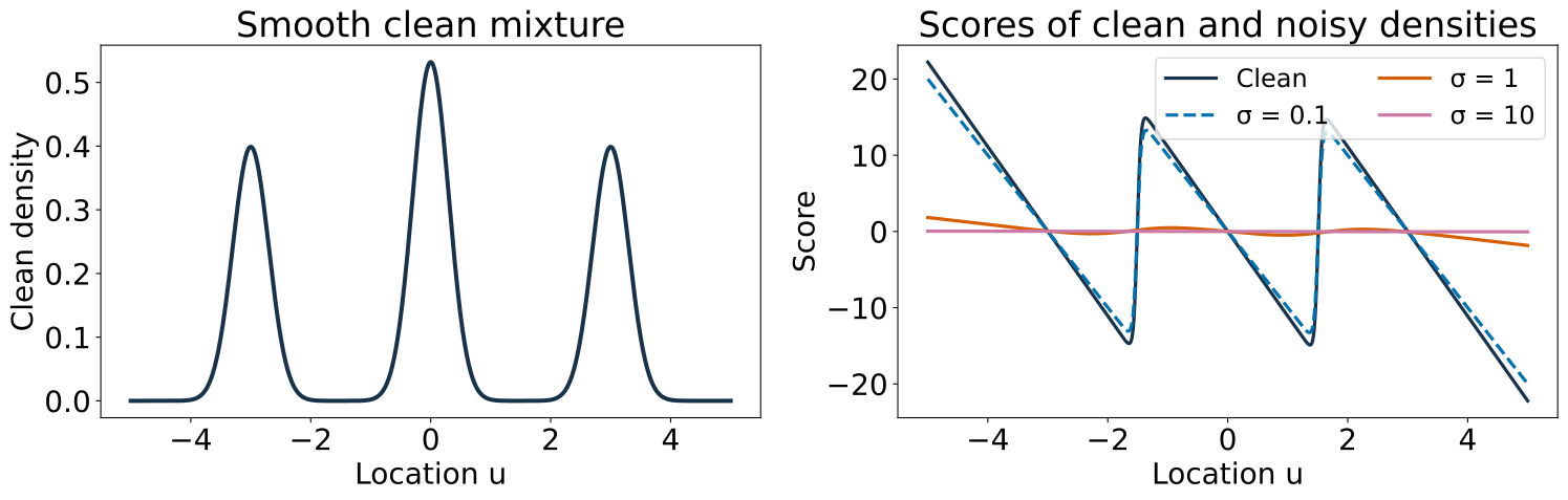
For a smooth positive clean density, under suitable regularity: \(\nabla\log p_\sigma(\widetilde{\boldsymbol{x}}_\sigma)\to\nabla\log p_{\mathrm{data}}(\widetilde{\boldsymbol{x}}_\sigma)\) as \(\sigma\to0\).

Three minutes. This is local convergence under smoothness/integrability and away from zeros of the clean density, not uniform control over all low-density regions. The smooth mixture from our running illustration supplies an example where the limit exists. A perfect circle is singular in2D and has no ordinary ambient clean log-density gradient; only its sigma>0 noisy scores are used in the next experiments. Even for a smooth density, limiting the ideal target does not guarantee learned accuracy where training inputs are rare. The clean-mixture score often has large magnitude in low-density gaps, but those gaps receive little training weight. [Sources] source:vincent-denoising-score-2011 for denoising score matching; original Gaussian-mixture limit calculation with explicit regularity qualification.

Small-noise training leaves poorly constrained scores away from data

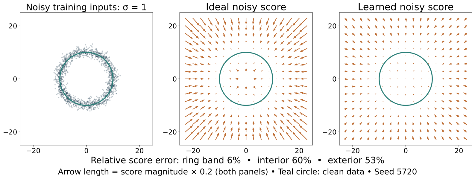
Clean data: uniform on a radius-10 circle. Train a small MLP at \(\sigma=1\).

Measured failure here: wrong magnitudes off the ring; directions mostly remain radial.

Three minutes. Actual neural training, not an analytic field relabeled learned. MLP2→64tanh→64tanh→2, input divided by10, output normalized noise; Adam lr.001,6000steps, batch512, newly drawn clean circle points and Gaussian noise each batch. Analytic values never enter training. First predeclared seed5720 is shown;5721/5722 also reported. On30000shared spatial points, relative vector-field RMSE is6.4% near ring8<r<12,60.1% interior r<6,52.6% exterior r>18. Mean angular errors, excluding near-zero ideal scores, are5.4°,2.4°,4.4° respectively; do not claim angular failure that this symmetric experiment did not show. All three seeds have approximately59–62% interior and51–53% exterior relative errors. Plot arrows preserve relative magnitudes using a stated common scale within the slide. Held-out noisy-data excess epsilon MSE per entry is.00333. Sparse training coverage leaves extrapolation weakly constrained; it does not force every architecture to point the wrong way. Original experiment; source:vincent-denoising-score-2011 supplies only the score/predictor relation.

Large noise improves coverage but changes the score being learned

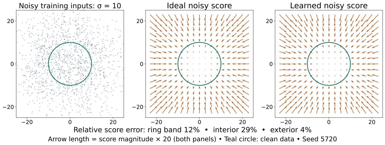
Same architecture and training budget, now \(\sigma=10\).

A good estimate of \(\nabla\log p_{10}\) is still not the clean-data score.

Three minutes. Same three seeds, optimizer, batch and steps; only corruption scale changes. First seed5720: field RMSE11.5% near ring,28.7% interior,4.4% exterior; angles4.3°,8.6°,1.8°. It improves broad-region magnitudes substantially relative to sigma1, not every metric in every region. Other seeds show the same qualitative coverage benefit. The exact radius10 sigma10 noisy density has an inward score for every nonzero radius. A correct fixed-noise Langevin sampler would target p10, not the clean circle; following the score deterministically would instead climb toward a mode, not sample either distribution. No claim that clean generation is impossible by every conceivable deconvolution method—this single-level sampling rule targets the noisy density. The next level must change the target score. Original measured experiment, no image-model evidence.

What would perfect single-level sampling produce?

Suppose the \(\sigma=10\) score is exact and the sampler correctly targets its density.

What would more accurate sampling recover?

A. The clean radius-10 circle

B. The broad noisy distribution \(p_{10}\)

C. One conditional-mean point

B. Better approximation cannot change the distribution the score describes.

Two minutes. Separates learning error, numerical error and target smoothing. A is tempting because training started from clean-circle examples; C confuses sampling with averaging or mode seeking. This motivates learning an entire sequence of noisy scores, reducing sigma during generation. Use p_sigma notation here: p10 means standard deviation10; the next section explicitly changes to p_t with variance-time t, where that same density is p100. Original transfer question.

Learning across noise levels

Broad coverage first; clean-data detail at lower noise

Twenty seconds. Move from the limitations of one level to a time-conditioned family, direct training draws and discrete reverse steps.

Multiple noise levels connect broad coverage to fine detail

Noisy scores → discrete noise levels → continuous SDE/ODE sampling

Now \(t\) denotes noise variance: \(\sigma_t=\sqrt t\), \(\widetilde{\boldsymbol{x}}_t=\boldsymbol{x}+\sqrt t\,\boldsymbol{\epsilon}\), and \(\widetilde{\boldsymbol{x}}_0=\boldsymbol{x}\).

1. Large noise: learn directions across a broad region.
2. Intermediate noise: change the target toward cleaner structure.
3. Small noise: resolve detail near the clean data.

Two minutes. This motivates a family of related denoising tasks and a matching reverse process. Now change indexing: sigma denotes noise standard deviation; t denotes accumulated variance, sigma=sqrt(t). Thus p_t in this section equals the preceding p_sigma at sigma=sqrt(t). Set tilde x_0=x. The parameter t will later become continuous. It is not a claim that arbitrary mean corrections sample the desired distribution.

Every time slice is a distribution over possible noisy samples

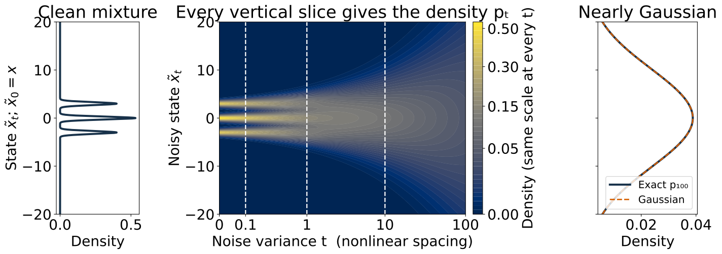
\[p_t(\widetilde{x}_t)=\sum_{j=1}^{3}w_j\,\mathcal N(\widetilde{x}_t;\mu_j,\,0.09+t),\qquad (\mu_1,\mu_2,\mu_3)=(-3,0,3).\]

Two minutes. Return to the smooth1D mixture used in the clean-score limit. Weights .3,.4,.3; small clean component SD.3. Horizontal time measures accumulated variance; nonlinear spacing preserves visible low-noise structure. Color is density under one fixed cividis shade/hue scale, not time and not a separate normalization per slice. A slice integrates to one over all real x; the plot crops tails. At t100 the single Gaussian overlay has variance105.49, the exact marginal variance, and closely approximates p100. Do not call the exact finite-time mixture Gaussian. This same density and fixed analytic predictor recur in reverse paths, step decomposition and histogram checks. Original analytic construction; source:song-score-sde-2021 for time-indexed marginals.

Independent standard-normal steps make noise variance add

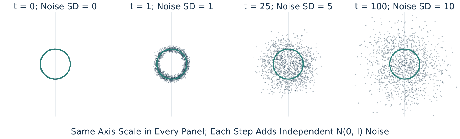
\[\widetilde{\boldsymbol{x}}_t=\widetilde{\boldsymbol{x}}_{t-1}+\boldsymbol{\eta}_t, \qquad\boldsymbol{\eta}_t\overset{\mathrm{iid}}{\sim}\mathcal N(\boldsymbol0,I).\]

After \(t\) steps: noise variance \(t\); noise standard deviation \(\sqrt t\).

Three minutes. Instructor-requested additive walk, matching the earlier offering. The circle now has radius10, so one standard-normal step (noise SD1) is small relative to the data scale and matches the small-noise example. At t100 the noise SD10 matches the large-noise example. Every panel has the same axis limits; these are intermediate forward states, not a claim that the last panel is already a Gaussian endpoint. Use T much larger than R^2=100 when relying on a noise-dominated initialization. Gaussian increments are independent of the clean point and each other. The residual final-step posterior has finite uncertainty even at this larger radius; a mean prediction is still not an exact clean-data sample.

Any noisy training input needs only one Gaussian draw

\[p_t(\widetilde{\mathbf{x}}_t\mid\boldsymbol{x})=\mathcal N(\widetilde{\mathbf{x}}_t;\boldsymbol{x},tI), \qquad \widetilde{\boldsymbol{x}}_t=\boldsymbol{x}+\sqrt t\,\boldsymbol{\epsilon}, \quad\boldsymbol{\epsilon}\sim\mathcal N(\boldsymbol0,I).\]

• Independent Gaussian variances add: \(I+\cdots+I=tI\).
• Select \(t\) and construct its noisy input directly.
• For large \(T\), the noise dominates: start generation approximately from \(\mathcal N(\boldsymbol0,TI)\).

Three minutes. Epsilon here represents normalized accumulated noise, not the final incremental eta_t. The direct draw matches a marginal, not the joint law of an entire trajectory. The terminal distribution is the convolution of the data distribution with N(0,TI), not exactly a Gaussian. N(0,TI) is a useful approximation when data magnitude is small relative to sqrt(T); center data for this simple initialization. For the circle, x_T/sqrt(T) approaches N(0,I) as T grows, whereas x_T itself grows in scale. No alpha, beta, or signal-shrink factor is used in this parameterization.

One network learns noise prediction at every level

Add the noise level to the input: \(\widehat{\boldsymbol{\epsilon}}_i=\epsilon_\theta(\widetilde{\boldsymbol{x}}_{t_i},t_i)\).

Step	Computation for each image in a batch
Draw level and noise	\(t_i\sim\operatorname{Uniform}\{1,\ldots,T\}\), \(\boldsymbol{\epsilon}_i\sim\mathcal N(\boldsymbol0,I)\)
Construct input	\(\widetilde{\boldsymbol{x}}_{t_i}=\boldsymbol{x}_i+\sqrt{t_i}\,\boldsymbol{\epsilon}_i\)
Predict and score	\(\widehat J=\frac1B\sum_i\|\boldsymbol{\epsilon}_i-\epsilon_\theta(\widetilde{\boldsymbol{x}}_{t_i},t_i)\|^2\)
Update shared parameters	\(\theta\leftarrow\theta-\eta\nabla_\theta\widehat J\)

One sampled level per image; the same parameters across levels.

Three minutes. Same fixed-level algorithm as before, now with an independent level for each example and an explicit time input. Tensor shapes remain batch-first. This is a simple noise-MSE objective, not a claim of exact ELBO equality. The clean estimate is tilde x_t-sqrt(t)epsilon_theta. Unweighted noise MSE corresponds to clean squared error weighted by1/t. The radius10 circle makes the t1 noise small relative to the radius while retaining unit-variance increments. A finer time grid is possible but is not needed to explain this example. The final conditional mean still has a small inward bias. [Sources] source:ho-ddpm-2020, algorithm1 for the training pattern, adapted to the explicitly different additive walk.

Reverse generation needs small conditional steps, not one clean guess

A clean-image estimate uses the whole predicted noise:

\[\widehat{\boldsymbol{x}}=\widetilde{\boldsymbol{x}}_t-\sqrt t\,\epsilon_\theta(\widetilde{\boldsymbol{x}}_t,t).\]

For the additive walk, the previous-step conditional mean instead uses

\[\widehat{\boldsymbol{\mu}}_{t-1}=\widetilde{\boldsymbol{x}}_t- \frac{1}{\sqrt t}\epsilon_\theta(\widetilde{\boldsymbol{x}}_t,t).\]

Generation follows \(T\to T-1\to\cdots\to0\) with fixed learned parameters.

A mean is not a full distribution: a reverse sampler must also handle uncertainty.

Four minutes. This closes the opening and sets up the reverse-sampler continuation, rather than silently reusing the incompatible variance-preserving DDPM formula. For t>1 Gaussian conditioning gives p(x_(t-1)|tilde x_t,clean x)=N(((t-1)/t)tilde x_t+clean x/t,((t-1)/t)I). Averaging over clean x conditional on tilde x_t gives E[x_(t-1)|tilde x_t]=tilde x_t-(tilde x_t-E[clean x|tilde x_t])/t, hence the displayed formula with an ideal normalized-noise predictor. The unconditional reverse conditional is generally a mixture, not exactly Gaussian: its covariance is ((t-1)/t)I+Cov(clean x|tilde x_t)/t^2. Adding only the bridge variance to this averaged mean is not generally exact. At t1 the true posterior on clean circle points remains uncertain, whereas its mean lies inside the circle. The next shared partial develops fine-step stochastic reverse approximations and their endpoint treatment. Do not present these conditional-mean equations alone as a complete exact sampler. Original derivation for the additive process; source:ho-ddpm-2020, section2 provides the related Gaussian forward/reverse modeling framework with a different schedule.

A stochastic reverse step denoises, then adds fresh noise

Move from current noise variance \(t\) to a lower variance \(s\geq0\). The step size is \(h=t-s>0\): how much we reduce the noise variance.

A DDPM-style step in our additive units is

\[\widetilde{x}_s=\underbrace{\widetilde{x}_t-\frac{h}{\sqrt t}\epsilon_\theta(\widetilde{x}_t,t)}_{m:\ \text{previous-level mean}} +\underbrace{\sqrt{\frac{sh}{t}}\,\xi}_{\text{fresh noise}},\qquad \xi\sim\mathcal N(0,1).\]

• The correction uses \(h/t\) of the predicted clean-data correction.
• For small \(h\) relative to \(t\), the added variance is approximately \(h\).
• This Gaussian step approximates the reverse conditional distribution.

Three minutes. Conditional on both tilde x_t and clean x, the Gaussian bridge variance is sh/t and its mean is (s/t)tilde x_t+(h/t)clean x. Replacing clean x by its conditional mean yields the displayed mean but omits the extra reverse variance (h/t)^2 Var(clean x|tilde x_t). The exact reverse conditional is generally a mixture. This is the fixed-small-variance DDPM construction expressed in additive units; it is not an exact finite-step sampler even with ideal epsilon. In Ho’s units z_t=sqrt(alpha_bar_t)clean x+sqrt(1-alpha_bar_t)epsilon, divide z_t by sqrt(alpha_bar_t) and use t=(1-alpha_bar_t)/alpha_bar_t. Then the rescaled noise coefficient is sqrt(s(t-s)/t). The paper’s index and our variance-time t differ. At s0 the variance vanishes and the last mean is still an approximation. [Sources] source:ho-ddpm-2020, section3.2; source:song-ddim-2021, equation12; source:song-score-sde-2021, reverse-SDE limit.

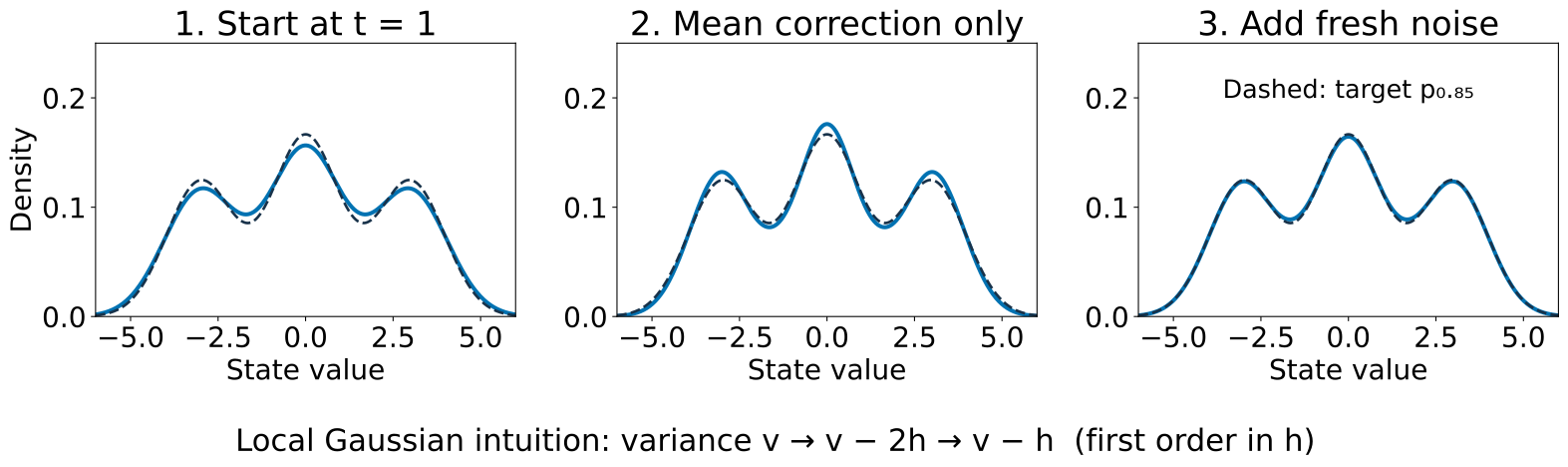
Mean correction narrows the distribution; noise spreads it again

“Denoise two, add back one” describes local variance change—not a time reversal.

Two minutes. The middle distribution is an algorithmic intermediate, not p at a hidden earlier time. For one local Gaussian of total variance v, the mean map multiplies deviations by 1-h/v, giving v-2h+h^2/v; independent step noise adds sh/t, approximately h. Net variance is v-h to first order. This gives the requested two-down/one-back intuition, not exact global movement between p_t slices. One random draw may move either direction in x; t still moves only from t to s. Diagram uses the exact push-forward density of the mean map then Gaussian convolution, so its small mismatch from the dashed target is real finite-step error. [Sources] source:song-score-sde-2021, equations6/13; original mixture calculation and first-order Gaussian illustration.

Diffusion as a continuous process

From Gaussian steps to SDEs and continuous-time training

Twenty seconds. The discrete step is already concrete. Now introduce Brownian increments, easy marginal training and the reverse SDE.

Continuous noising is the small-step limit of the Gaussian walk

Discrete diffusion → continuous SDE → probability-flow ODE → solver choices

\[d\widetilde{\boldsymbol{x}}_t=d\mathbf{w}_t,\qquad \widetilde{\boldsymbol{x}}_0=\boldsymbol{x}.\]

• An SDE adds random increments: \(\Delta\mathbf{w}\sim\mathcal N(\boldsymbol0,hI)\) over an interval \(h\).
• Our time label is noise variance: \(\sigma(t)=\sqrt t\).
• Its marginal remains \(\widetilde{\boldsymbol{x}}_t=\boldsymbol{x}+\sqrt t\,\boldsymbol{\epsilon}\) in distribution.

Two minutes. Brownian w is a random vector-valued process; its finite increments are independent Gaussians with covariance hI. SDE means stochastic differential equation. This is the additive/variance-exploding example, not the most general diffusion. A marginal draw formula is not a coupled path obtained by keeping the same epsilon for all times. General forward SDEs have f(x,t)dt+g(t)dw; standard linear Gaussian VP/VE choices have tractable conditional marginals. We retain our additive choice to keep all figures and coefficients consistent. [Sources] source:song-score-sde-2021, section3; source:karras-edm-2022, section2.